Faulty LED Display Digit Recognition: Illustration of Naive Bayes Classifier using Excel

Originally published on July 17, 2017.

The Naive Bayes (NB) classifier is widely used in machine learning for its appealing tradeoffs in terms of design effort and performance as well as its ability to deal with missing features or attributes. It is particularly popular for text classification. In this blog post, I will illustrate designing a naive Bayes classifier for digit recognition where each digit is formed by selectively turning on/off segments of a seven segment LED display arranged in a certain fashion as shown below. The entire exercise will be carried out in Excel. By writing Excel formulas and seeing the results in a spreadsheet is likely to result in a better understanding of the naive Bayes classifier and the entire design process.

We will represent each digit as a 7-dimensional binary vector where a 1 in the representation implies the corresponding segment to be on. The representations for all ten digits, 0-9, is shown below. Furthermore, we assume the display to be faulty in the sense that with probability p a segment doesn't turn on(off) when it is supposed to be on(off). Thus, we want to design a naive Bayes classifier that accepts a 7-dimensional binary vector as an input and predicts the digit that was meant to be displayed.

Basics of Naive Bayes

A Naive Bayes (NB) classifier uses Bayes' theorem and independent features assumption to perform classification. Although the feature independence assumption may not hold true, the resulting simplicity and performance close to complex classifiers offer complelling reasons to treat features to be independent. Suppose we have $d$ features, $x_1,\cdots, x_d$, and two classes $ c_1\text{ and } c_2$. According to Bayes' theorem, the probability that the observation vector $ {\bf x} = [x_1,\cdots,x_d]^T$ belongs to class $ c_j$ is given by the following relationship:

$ P(c_j|{\bf x}) = \frac{P(x_1,\cdots,x_d|c_j)P(c_j)}{P(x_1,\cdots,x_d)}, j= 1, 2$

Assuming features to be independent, the above expression reduces to:

$ P(c_j|{\bf x}) = \frac{P(c_j)\prod_{i=1}^{d}P(x_i|c_j)}{P(x_1,\cdots,x_d)}, j= 1, 2$

The denominator in above expression is constant for a given input. Thus, the classification rule for a given observation vector can be expressed as:

Assign

$ {\bf {x}}\rightarrow c_1\text { if }P(c_1)\prod_{i=1}^{d}P(x_i|c_1)\geq P(c_2)\prod_{i=1}^{d}P(x_i|c_2)$

Otherwise assign

$ {\bf {x}}\rightarrow c_2$

For classification problems with C classes, we can write the classification rule as:

$ {\bf {x}}\rightarrow c_j \text{ where } P(c_j)\prod_{i=1}^{d}P(x_i|c_j) > P(c_k)\prod_{i=1}^{d}P(x_i|c_k), k=1,...,C \text{ and } k\neq j$

In case of ties, we break them randomly. The implementation of the above classification rule requires estimating different probabilities using the training set under the assumption that the training set is a representative of the classification problem at hand.

There are two major advantages of the NB classification when working with binary features. First, the naive assumption of feature independence reduces the number of probabilities that need to be calculated. This, in turn, reduces the requirement on the size of training set. As an example, consider the number of binary features to be 10. Without the naive independence assumption, we will need to calculate $ 2^{10}$ (1024) probabilities for each class. With the independent features assumption, the number of probabilities to be calculated per class reduces to 10. Another advantage of NB classification is that it is still possible to perform classification even if one or more features are missing; in such situations the terms for missing features are simply omitted from calculations.

Faulty Display Digit Recognition Steps

In order to design a classifier, we need to have training data. We will generate such data using Excel. To do so, we first enter the seven dimensional representation for each digit in Excel and name the cell ranges for each digit as digit1, digit2 etc. as shown below.

Next, we use Excel's RAND() function to decide whether the true value of a segment should be flipped or not (1 to 0 or 0 to 1). We repeat this as many times as the number of training examples for each digit need to be generated. In discussion here, we will generate 20 examples for each digit. The figure below shows some of the 20 such examples and the Excel formula used to generate them for digit 1. Noiselevel in the formula refers to a cell where we store the probabilty p of a segment being faulty. This value was set to 0.2. Similar formulas are used to generate 20 examples for each digit.

The 200 training examples generated as described are next copied and pasted into a new worksheet. This is the sheet that will be used for designing the classifier. The paste operation is carried out using the "Values Only" option. This is done to avoid anymore changes in the generated noisy examples.

Naive Bayesian Classifier Design

Having generated 200 examples of faulty display digits, we are now ready to design our NB classifier. Designing NB classifier means we need to compute/estimate class priors and conditional probabilities. Class priors are taken as the fraction of examples from each class in the training set. In the present case, all class priors are equal. This means that class priors do not play any role in arriving at the class membership decision in our present example. Thus, we need to estimate only conditional probabilities. The conditional probabilities are the frequencies of each attribute value for each class in our training set. The following relationship provides us with the probability of segment 1 being equal to 1 conditioned on that the digit being displayed is digit 1.

$P(s_{1}=1|digit1) = \frac{\text{count of 1's for segment 1 in digit1 training examples}}{\text{number of digit1 training examples}}$

Since only two possible states, 1 and 0, are possible for each segment, we can calculate the probability of segment 1 being equal to 0 conditioned on that the digit being displayed is digit 1 by the following relationship:

$ P(s_{1}=0|digit1) = 1 - P(s_{1}=1|digit1)$

In practice, however, a correction is applied to conditional probabilities calculations to ensure that none of the probabilities is 0. This correction, known as Laplace smoothing, is given by the following relationship:

$ P(s_{1}=1|digit1) = \frac{1+\text{count of 1's for segment 1 in digit1 training examples}}{2+\text{number of digit1 training examples}}$

Adding 1 to the numerator count ensures probability value doesnot become 0. Adding 2 to the denominator reflects the number of states that are possible for the attribute under consideration. In this case we have binary attributes. Note that in text classification applications, for example in email classification, where we use words in text as attributes, the denominator correction term will be V with V being the number of words in the dictionary formed by all words in the training examples. Also you will find the term Bernoulli NB being used when the feature vector is a binary vector as in the present case, and the term Multinomial NB being used when working with words as features.

Going back to our training set, we are now ready to compute conditional probabilities. The formula for one such computation is shown below along with a set of training examples for digit1. Similar formulas are used to compute the remaining conditional probabilities and the training examples to obtain 70 conditional probabilities needed to perform classification.

Testing the Classifier

Having calculated conditional probabilities, we are now ready to see how well our classifier will work on test examples. For this, we first generate five test examples for each digit following the steps outlined earlier. The test examples are copied and pasted (using the "Value Only" paste option). We also copy the probabilties computed above to the same worksheet where test examples have been pasted, just for convenience. This done, we next write formulas to compute the probabilty for each digit given a test example and the set of conditional probabilities. This is shown below in a partial screenshot of Excel worksheet where the formula shown for calculating the probability of displayed digit being 1 based on the states of seven segments. The references to cells in the formula are where we have copied the table of conditional probabilities.

While the higlighted columns indicate the highest probability value in each row and thus the classification result, the following formula in column "S" results in the classifier output as the label to be assigned to the seven component binary input representing the status of the faulty display.

=MOD(MATCH(MAX(I2:R2),I2:R2,0),10)

Next, comparing the labels in columns H (true label) and S (predicted label) we can generate the confusion matrix to tabulate the performance of the classifier. Doing so results in the following confusion matrix with 80% correct classification rate.

The 80% accuracy is for 20% noise level. If desired we can go back and rerun the entire simulation again for different noise levels and determine how the accuracy varies with varying noise levels.

Finally, it would be nice to have a visual interface where we can input a row number referencing a test example, and display the faulty digit as well as the predicted digit. Such a display can be easily created using conditional formatting and adjusting the shape and size of certain Excel cells (See a post on this). One such display is shown below. By entering a number in the range of 2-51 (50 test examples) in cell AE1, we can pull out the segment values using Indirect function of Excel. For example, the segment value shown in cell W3 in figure below is obtained by the following formula =INDIRECT("A"&$AE$1). Similary, the value in cell X3 is obtained by =INDIRECT("B"&$AE$1), and so on. The segment values in the cell range W3:AC3 are then used in conditional formatting. The predicted digit display is based on segments states corresponding to the predicted digit label read from "S: column for the row number in AE2.

As this exercise demonstrates, the design of a naive Bayes classifier is pretty straightforward. Hopefully working with Excel has provided a better understanding of the steps involved in the entire process of developing a classifier. 

Gradient Boosted Regression and Classification Trees

 A long while ago I had posted about how a "A Bunch of Weak Classifiers Working Together Can Outperform a Single Strong Classifier." Such a bunch of classifiers/regressors is called an ensemble. As mentioned in that post, bagging and boosting are two techniques that are used to create an ensemble of classifiers/regressors. In this post, I will explain how to build an ensemble of decision trees using gradient boosting. Before going into the details, however, let us first understand boosting, gradient boosting, and why the decision tree classifiers and regression trees are the most suitable candidates for creating an ensemble.

The individual units in an ensemble are known as weak learners. Such learners are brittle in nature, i.e. a small change in the training data can have a major impact on their performance. This brittle nature helps to ensure that the weak learners are not well-correlated with each other. The choice of the tree model for weak learners is popular because tree models exhibit decent brittleness and such models are easily trained without much computation effort.

Boosting is one technique to combine weak learners to obtain a single strong learner or model. Bagging is another such technique. In bagging, all weak learners learn in parallel and independent of other learners. Every learner in bagging looks at only a part of the training data or a subset of features or both. In boosting, the weak learners are build sequentially using the full training data and the results from the preceding weak learners. Thus, boosting builds an additive model and the output of the ensemble is taken as the weighted sum of the predictions of the weak learners.

In the original boosting algorithm AdaBoost, the successive weak learners try to improve the accuracy by giving more importance to those training examples that are misclassified by the prior weak learners. In gradient boosting, the results from the preceding weak learners are compared with the desired output to obtain a measure of the error which the next weak learner tries to minimize. Thus, the focus in gradient boost is on the residuals, i.e. the difference between the desired output and the actual output, rather than on those specific examples that were misclassified by the earlier learners. The term gradient is used because the error minimization is carried out by using the gradient of the error function. The sequence of successive trees are of identical depth from 1 (stump) to 4.

A Walk Through Example to Build a Gradient Boosted Regression Tree

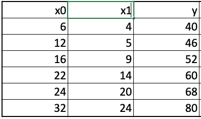
Let us work through an example to clearly understand how gradient boosted trees are build. We will take a regression example because building a gradient boosted regression tree is easier to understand than a gradient boosted classification tree. The example consists of two predictors, fertilizer input (x0) and insecticide input (x1), and the output variable is the crop yield (y). The goal is to build a gradient boosted regression tree to predict the crop yield given the input numbers for x0 and x1.

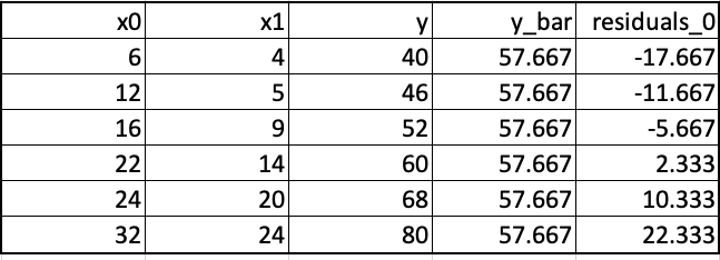
We will build a tree that minimizes the squared error (mse) between the actual output and the predicted output. We begin by building a base learner that yields the same prediction irrespective of the values of the predictor variables. This base prediction, let us denote it as y_hat_0, equals average of the output variable y, y_bar. Next, we calculate the residuals, the difference between the actual output y and the predicted output to obtain the residuals as shown below.

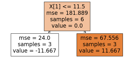
The next step is to adjust the predictions by relating the residuals with x0 and x1. We do this by fitting a regression tree to the residuals. We will use a tree of depth 1. To build the tree, we find the feature and the cut-off or the threshold value that best partitions the training data to minimize the mean squared error (mse). For the root node, such a combination consists of predictor x1 and the cut-off value of 11.5. The resulting tree is shown below. This tree was build using the DecisionTreeRegressor of the Sklearn library. Let's look at the meanings of different entries shown in the tree diagram. The mse value of 181.889 in the internal node of the tree is nothing but the error value if the residuals_0 column is approximated by the column average which is being shown by "value = 0." The number of examples associated with a node in the tree is given by "samples."

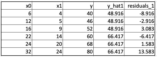
The above tree shows residual approximation by -11.667 for those training examples whose x1 value is less than or equal to 11.5 and the approximation by 11.667 when x1 is greater than 11.5. Assuming a learning rate of 0.75, we combine the above tree with the base tree (stump) to obtain updated predictions and the next set of residuals as shown below. To understand how the updated predictions were calculated, consider the predictor variables x0=6 and x1=4. The above tree tells us that for x1=4, the residual should be approximated by -11.667. The previous prediction for this particular x0,x1 combination is 57.667. Thus, the new prediction in this case becomes 57.667+0.75*(-11.667) which equals 48.916.

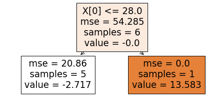
With the new set of residuals, we again build a tree to relate x0, x1 with residuals_1. This tree is shown below.

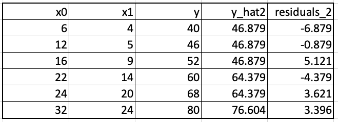
We update the predictions. For the first training example, the updating leads to the prediction 48.916+0.75*(-2.717) which equals 46.879. These updated predictions, y_hat2, and the new residuals, residuals_2 are shown below.

The tree building process continues in this fashion to generate either the specified number of weak learners or to the acceptable level of error.

Now that we know how gradient boosted trees are created, let us finish the above example using the GradientBoostingRegressor from the Sklearn library as shown below. The number of learners has been specified as 10 and the depth is set to 1.

import numpy as np from sklearn.ensemble import GradientBoostingRegressor from sklearn.metrics import mean_squared_error # Create data for illustration X = np.array([[6,4],[12,5], [16,9],[22,14],[24,20],[32,24]]) y = np.array([40, 46, 52, 60, 68,80]) regressor = GradientBoostingRegressor(     max_depth=1,     n_estimators=10,     learning_rate=0.75 ) gbt = regressor.fit(X, y) gbt.predict(X)

array([40.18852649, 46.37977649, 49.56846063, 62.91676214, 67.36073713,        79.58573713])

How about Gradient Boosted Classification Trees?

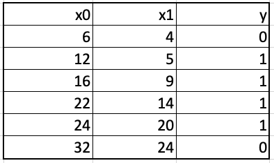
Let us convert the above regression example to a classification example by considering whether the crop yield was profitable or not based on fertilizer and insecticide costs. Thus, the output variable y now has two values, 0 (loss) and 1 (gain) as shown below.

Just like the procedure for building gradient boosted regression trees, we begin with a crude approximation for the output variable. The initial probability of class 1 over all the training examples, equal to 0.667, is taken as this approximation. The gradient boosted classifier is built using regression trees just like it is done while building gradient regression trees. The successive learners try to reduce the residuals, the difference between the y and the predicted probability.

Log Likelihood Loss Function and Log(odds)

The loss function minimized in the gradient boosted classification tree algorithm is the negative log likelihood. For a classification problem with two classes as we have, the negative log likelihood for the i-th training example is expressed by the following formula where p stands for the probability that the example is from class 1.

The loss is summed over all training examples to get the over all loss. The ratio p/(1-p) is called the odds or odds ratio, and often is expressed in terms of log(odds) by taking the natural log of the odds ratio. The probability p of an event and its log(odds) are related through the following equation:

Through some simple algebraic manipulation, we can also express the loss function as

Instead of calculating the gradient of the loss function with respect to p, it turns out that adjusting log(odds) offers a better way to minimize the loss function. Thus, taking the gradient of the loss function with respect to log(odd) results in the following expression:

The first term on the RHS of the equation is the negative of the desired output while the second term corresponds to the predicted probability (see the relationship between p and log(odds) above). The negative of the RHS in the above equation defines the residuals that we try to minimize by building successive trees via regression.

Back to Example

Coming back to our example, since the initial probability attached to every training example is 0.667 (ratio of class 1 labels and class 0 labels), the residuals are:

-0.667,  0.333,  0.333,  0.333,  0.333, -0.667

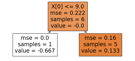
Let us try to fit a regression tree to the residuals at hand. Again, we will fit a tree of unit depth using the DecisionTreeRegressor from the Sklearn. The resulting tree shown below.

While in the case of the gradient regression trees, the "value" from the leaf nodes were directly used in the calculations of the updated residuals, we need to map "value" into log(odds) for calculating a new set of residuals in the present case. This mapping is done using the following relationship:

Let us try to understand the quantities in the RHS of the above expression. We will do so by referring to the right leaf node of the above tree. This leaf node has 5 samples that refer to the index "i" in the above expression. The item "value" in the leaf nodes is the residual for each example in the leaf node. There are five examples associated with the right leaf node; these are all but the first example of our data set. The previous probability is 0.667 for each of these examples. Thus, the mapped_log(odds) for these five examples are 5*0.133/(5*0.667*0.333), which equals 0.599. With 0.75 as the learning rate, the new log(odds) values for these five examples become 0.693(old log(odds)) + 0.75*(0.599) resulting in 1.142 for each of the five examples of the data set for which x0<9. Converting these log(odds) to probabilities, we see that 0.758 is the probability for the last five examples in the right leaf node to be from class 1. Carrying out similar calculations for the left leaf node, we end up with -1.559 as the updated log(odds) which translates to 0.174 as the probability that our first example in the data set is from class 1 or from the positive class.

Subtracting the updated probabilities from column y, we get a new set of residuals as shown below:

[-0.174,  0.242,  0.242,  0.242,  0.242, -0.758]

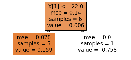
The regression tree built to fit these residuals is shown below.

We need to calculate the mapped_log(odds) again. The example associated with the right leaf in this case is the last example of the data set. The mapped log(odds) value for this example comes out as -4.132 following the formula for mapping shown above. The updated log(odds) value is then the 1.142(prior value) + 0.75* (-4.132). Converting the result into the probability, we get 0.123 as the probability that the last example in our data set comes from the positive class. Thus, it is classified as belonging to the negative (label 0) class. Let us now map the left leaf node value to log(odds) using the mapping formula.

= 5*0.159/((4*0.758*(1-0.758)+0.174*(1-0.174)))
= 0.906

This results in 0.906. Out of the five examples associated with the left leaf node, the four examples(all with y = 1) were together in the previous tree and had the updated log(odds) value 1.142 at that instance. The current log(odds) value for these four examples is then 1.142+0.75*0.906, equal to 1.821 which yields a probability value of 0.860. Thus, these four examples are correctly assigned the probability of 0.860 for the positive class. The remaining fifth example in the left node has a prior log(odds) value of -1.559. Thus, its updated log(odds) becomes -1.559+0.75*0.906, equal to -0.879. This gives 0.293 as the probability of this example from the positive class. Since the probability for the negative class is higher, this example is also correctly classified. At this stage, there is no need to add anymore learner because all examples have been correctly classified.

The above example was done to illustrate how the gradient boosted classifier builds its learners. Let us apply the GradientBoostingClassifier from the Sklearn library to check our step by step assembly of the learners explained above. We will print out the probability values to compare against our calculations.

from sklearn.ensemble import GradientBoostingClassifier clf = GradientBoostingClassifier(     criterion='mse', max_depth=1,     n_estimators=2,     learning_rate=0.75 ) gbdt = clf.fit(X, y) list(gbdt.predict_proba(X))

[array([0.70657313, 0.29342687]),
 array([0.13928973, 0.86071027]),
 array([0.13928973, 0.86071027]),
 array([0.13928973, 0.86071027]),
 array([0.13928973, 0.86071027]),
 array([0.87645946, 0.12354054])]

You can see that these probabilities are identical to those calculated earlier. Thus, you now know how to build a gradient boosted classifier.

Before You Leave

Let us summarize the post before you leave. Boosting relies on an ensemble of trees to perform regression and classification. The gradient boosted trees for regression and classification give excellent performance. Using the Sklearn library without paying much attention to the number of learners and tree depth can lead to over-fitting; so care must be taken. One disadvantage common to all ensemble methods is that the simplicity of understanding model that one gets using a single tree is lost. A speedier and more accurate and scalable version of gradient boosted trees is the extreme gradient boosted trees (XGBoost). The performance of XGBoost algorithm is at par with deep learning models and this model is very popular. 

Image

Insert an image to make a visual statement.

Settings

Alternative text

Describe the purpose of the image.(opens in a new tab)

Leave empty if decorative.

Aspect ratio

Width

px

Height

px

Scale

Resolution

Select the size of the source image.

Looking for other block settings? They've moved to the styles tab.

• Image

Linear Regression using ChatGPT

[Originally published on March 7, 2023]

The ChatGPT is a large language model (LLM) from OpenAI that was released a few months ago. Since then, it has created lots of excitement in terms of a whole range of possible uses for it, lots and lots of hype, and a lot of concern about harm that might result from its use. Within five days after its release, the ChatGPT had over one million users and that number has been growing since then. The hype arising from ChatGPT is not surprising; the field of AI from its inception has been hyped. One just need to be reminded of the Noble Prize winner Herbert Simon’s statement “Machines will be capable, within twenty years, of doing any work that a man can do” made in 1965. Several concerns about the potential harm due to ChatGPT’s use have been expressed. It has been found to generate inaccurate information as facts that is presented very convincingly. Its capabilities are so good that Elon Musk recently tweeted “ChatGPT is scary good. We are not far from dangerously strong AI.”

Since ChatGPT’s release, many companies and researchers have been playing with its capabilities and this has given rise to what is being characterized as Generative AI. It has been used to write essays, emails, and even scientific articles, prepare travel plans, solve math problems, write code and create websites among many other usages. Many companies have incorporated it into their Apps. And of course, Microsoft has integrated it into its Bing search engine.

Given all the excitement about it, I decided to use it to build a linear regression model. The result of my interaction with the ChatGPT are presented below. The complete interaction was over in a minute or so; primarily slowed by my one finger typing.

So, all it took to build the regression model was to feed the data and let the ChatGPT know the predictor variables. Looks like a great tool. But like any other tool, it needs to be used in a constructive manner. I hope you like this simple demo of ChatGPT’s capabilities. I encourage you to try on your own. OpenAI is free but you will need to register.