Understanding Knowledge Graphs - What They Are and How to Build Them

Knowledge graphs are a way to represent information and relationships between the real world entities, i.e. objects, events, facts etc., in a structured, interconnected way. They provide a powerful framework for capturing the rich semantics and context of data. Knowledge graphs are also called semantic networks.

At its core, a knowledge graph is a type of data model that structures information as entities (nodes) and their relationships (edges). Entities represent real-world objects like people, places, concepts, or events, while the relationships define how these entities are linked. An example of a small knowledge graph is shown below.

Some key characteristics of knowledge graphs are:

- Entities have properties that describe their attributes (e.g. name, date of birth for a person)

- Relationships have types that define how entities are connected (e.g. bornIn, employedBy)

- They provide context by capturing how pieces of data relate to one another

- Information is stored in a graph structure rather than tables


This graph-based approach provides flexibility in modeling complex, multi-dimensional data in a way that can be easily extended as new information emerges.

Applications of Knowledge Graphs

Knowledge graphs have broad applications across many domains:

- Search engines like Google use knowledge graphs to enhance search results with contextualized information
- Recommendation engines leverage knowledge graphs to provide relevant suggestions based on user preferences and behaviors  
- Biomedical research uses knowledge graphs to represent relationships between diseases, genes, drugs, and more
- Enterprise knowledge graphs help organizations better understand their data assets and how different systems/processes are interconnected

How to Build a Knowledge Graph

There are generally five key steps in creating a knowledge graph:

1. Data Ingestion - Gathering data from various structured and unstructured sources  
2. Entity Extraction - Identifying real-world entities mentioned in the data using techniques like named entity recognition (NER)
3. Relationship Extraction - Determining relationships between entities using methods like pattern matching or machine learning
4. Data Transformation - Converting the extracted triples (entity-relationship-entity) into the proper graph data model format
5. Graph Population - Loading the transformed data into the graph database

There are many different knowledge graph construction toolkits and frameworks available depending on your use case and data needs. Some popular open source options include:

- Stanford's CoreNLP for NLP processing 
- OpenKBC for end-to-end knowledge graph creation
- Python libraries like rdflib and owlready2 for working with semantic web standards

Knowledge graphs unlock new opportunities for data integration, analysis, and discovery. As our ability to capture, process, and connect information continues growing, knowledge graphs will become an increasingly vital tool.

What is Neuro-Symbolic AI and Why do we Need it?

Neuro-symbolic AI, also known as symbolic neural integration or hybrid AI, has been in news lately. It is an approach that combines symbolic reasoning and neural networks to create more robust and flexible artificial intelligence systems. This integration aims to leverage the strengths of both symbolic and neural approaches, addressing some of the limitations each paradigm faces independently.

Let's look at the following image to understand the need for the neuro-symbolic approach. The deep learning model looking at the input image comes to a conclusion that the image depicts a cow that is 5.2 meter long. Obviously, the system has been trained to recognize cows and other objects but is unable to reason that cows are not that long. This is not surprising as deep learning models are excellent at recognizing features but have no capability to understand or draw conclusions based on the spatial relationships between the detected features. One way to provide such capabilities is to integrate symbolic reasoning along with the feature detection and pattern recognition capabilities of deep neural networks, and thus the interest in the neuro-symbolic approach. 

#object detection #neuro-symbolic

The ways Neuro-Symbolic AI can help

  1. Improved Reasoning: Integrating symbolic reasoning with neural networks can enhance AI's ability to understand and apply common sense knowledge, making it more adept in real-world scenarios.
  2. Medical Diagnosis: Neuro-symbolic approaches can be applied to medical diagnosis, where symbolic rules can be used to represent expert knowledge, and neural networks can learn from diverse patient data to improve diagnostic accuracy.
  3. Robotics and Autonomous Systems: Combining symbolic reasoning with neural networks can enhance the decision-making capabilities of robots, allowing them to navigate complex environments and handle uncertainty.
  4. Natural Language Understanding: Neuro-symbolic AI can be used to improve natural language understanding systems by combining semantic representation with the ability to learn from diverse textual data.
  5. Financial Fraud Detection: Integrating symbolic rules for detecting fraud patterns with neural networks that can adapt to new, emerging fraud trends can enhance the accuracy and robustness of fraud detection systems

Challenges and Approaches

Integrating the neural and symbolic components in a principled and effective way remains a key challenge in neuro-symbolic AI. Several promising approaches are being explored:
  1. Neural Networks with Symbolic Inductive Biases: This approach aims to build neural architectures with inductive biases derived from symbolic AI, such as logical operations, algebraic reasoning, or compositional structure. For example, graph neural networks can inject relational inductive biases, while neural programmer-interpreters combine neural modules with program-like operations.
  2. Augmenting Neural Models with External Memory/Reasoning: Rather than directly encoding symbolic knowledge in the neural architecture, another approach uses external memory or reasoning components that interact with a neural network. Examples include memory augmented neural networks, neural semantic encoders, and neural-symbolic concept learners.
  3. Differentiable Inductive Logic Programming: Inspired by inductive logic programming (ILP) in symbolic AI, this approach uses neural networks to learn first-order logic rules or program-like primitives in a differentiable way that integrates symbolic reasoning into end-to-end training.
  4. Learning Symbolic Representations from Data: Techniques in this area aim to have neural networks automatically learn disentangled, symbolic-like representations from raw data in an unsupervised or self-supervised manner. Examples include sparse factor graphs, conceptor-based models, and neuro-symbolic concept invention.

For Further Exploration

You can check the following links for further exploration of this topic:
Despite progress, several key challenges remain, including scaling symbolic reasoning, imposing harder constraints in neural architectures, achieving systematic compositionality, and maintaining interpretability as models get larger. Hybrid neuro-symbolic approaches hold promise but will require significant research efforts across multiple fields.

More on Distances between Graphs

In an earlier post, I had mentioned the need for comparing graphs for different applications and described the spectral graph distance for the said purpose. In this post, we are going to consider two other graph distance measures. The first measure is called DeltaCon measure. This measure works under the assumption that the node correspondence between the two graphs is known. The second measure is known as the Portrait Divergence and can be used for any graph pair. In addition to these two measures, there are a few other measures that are available. It turns out that most measures yield highly correlated results; thus knowing 2-3 different measures is a good starting point to explore other measures as well as the applications where such measures are used.

DeltaCon Measure of Graph Similarity

The basic idea behind this method is to calculate an affinity measure between a pair of nodes in the first graph, repeat the similar affinity calculations for the corresponding node pair in the second graph, and then compare the two measures to get an idea about the difference in the node pairs over two graphs. By repeating the node affinity calculations over all node pairs for the respective graphs, one can get an aggregate measure for similarity between the two graphs. The pairwise node affinity s_{ij} between node I and node j is measured by looking at all possible paths between the two nodes. The DeltaCon paper shows that the similarity matrix S of a graph G measuring the similarity between different node pairs can be obtained by the following expression:

S = [s_{ij}] = [I + \epsilon^2 D - \epsilon A]^{-1},

where I is an identity matrix, D is the degree matrix, and A is the adjacent matrix of the graph G. The quantity \epsilon is a small positive constant.Given two graphs G^1 and G^2, the DeltaCon distance measure is computed using the following relationship:
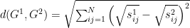
d(G^1,G^2) = \sqrt{\sum_{ij=1}^N\Big(\sqrt{s_{ij}^1}- \sqrt{s_{ij}^2}\Big)^2}

While the two similarity matrices can be compared using some other difference measure, the above DeltaCon measure is a true metric satisfying the triangular inequality of a true distance.

Illustration of DeltaCon Measure

Let’s use DeltaCon measure to compute distances between a set of graphs. We will do this using the netrd library which provides a NetworkX-based interface to compute various graph distances along with many other graph utilities. We will use the Air Transportation Multiplex Dataset for experimentation. The dataset is composed of a multiplex network composed of the airlines operating in Europe. It contains thirty-seven different layers of networks each one corresponding to a different airline. We will use only two subsets of the dataset consisting of the three biggest major airlines (Air France, British Airways, and Lufthansa),  and the three low-cost airlines (Air Berlin, Easy Jet, and Ryanair). A graph of the Ryanair is shown below; it consists of 149 nodes with 729 edges.

Ryanair Network
All the nodes in the dataset have an associated airport code and node indices are consistent over the entire multiplex. Thus, the node correspondence exists in the dataset. However, each airline flies to only a subset of the total nodes in the multiplex. Since DeltaCon requires node correspondence as well the same number of nodes in the two graphs to compare, we need to add nodes to the graphs under comparison to bring them to same size. The following code snippet shows how the DeltaCon distance is being computed for a pair of airlines; similar computation applies to other airline pairs.

import numpy as np
import networkx as nx
import netrd 

f = nx.read_adjlist(France.txt)
Fr = nx.Graph(f)
b = nx.read_adjlist(Brit.txt)
Br = nx.Graph(b)
list1 = list(Fr.nodes)
list2 = list(Br.nodes)
new_list1=set(list1)-set(list2)#Elements of list 1 that are not present in list 2
new_list2=set(list2)-set(list1)#Elements of list 2 that are not present in list 1 
Fr.add_nodes_from(new_list2)
Br.add_nodes_from(new_list1)
# Now both graphs have identical size and nodes are in correspondence
dist = netrd.distance.DeltaCon()
print(dist(Fr,Br))
1.5233983011182537

The figure below shows the distances between the networks of different airlines calculated using the DeltaCon measure. I applied the single linkage clustering to the resulting distance. The result shown below in the form a dendrogram puts the three major airlines in one cluster and the three low-cost airlines in another cluster. This suggests that the DeltaCon distance is able to capture the underlying properties of a graph and can be used for graph discrimination.

Distance matrix and Dendrogram by using DeltaCon

Portrait Divergence

This measure is based upon a matrix, called network portrait, which captures the distribution of shortest path lengths in a graph. The elements of the network portrait matrix $B$ for a graph with N nodes are defined as

$b_{j,k} \equiv \text{the number of nodes who have k nodes at distance j}$,

$ \text{ for } 0 ≤ j  ≤ D \text{ and } 0 ≤ k ≤ N − 1$. The distance is taken as the shortest path length and D refers to the graph diameter(length of the longest shortest path). The network portrait provides a concise topological summary of a graph and has the graph invariant property, and thus can be used for comparing two networks or graphs.

The portrait divergence measure is computed by treating the rows of the network portrait matrix B as probability distributions. These probability distributions are combined to create a single joint distribution for all rows. Given two graphs, the corresponding distributions are then compared using the Jensen-Shanon divergence measure to produce a similarity value in the range of 0-1. Please see for details.

Let’s see if the results given by this method are different from above or not by applying the portrait divergence measure to the airlines data. The results are shown below; these are similar and yield two similar clusters.

Distance matrix and Dendrogram by using Portrait Divergence

Takeaway

I have discussed only three methods for graph comparison, spectral graph distance (in an earlier blog post) and the two discussed in this post. The DeltaCon method requires prior knowledge about the graphs in terms of node to node mappings over the graph pair being compared. The spectral graph distance and the portrait divergence methods do not have any such requirement. As I indicated earlier, there are a few other distance measures for graph comparison; however all these measures yield correlated results. I suggest looking at this paper if you get interested in this topic as a result of this post.


Measuring Distance between Two Graphs

Graph-based representation is a natural choice in many areas such as biology, computer science, communication, social sciences, and telecommunication. Such representations are also known as network models. Often, we are interested in finding out how much different the two graphs are and want to specify that difference in the form of a numerical measure such as the distance or similarity between a pair of graphs. Measuring the distance between two graphs is different from the graph isomorphism problem where we look for a mapping based on one-to-one correspondence between the nodes of the two graphs. In this blog post, I am going to describe the graph distance measure, spectral graph distance, which has been suggested and used to measure the difference between a pair of graphs. In the subsequent blog posts, I intend to describe some other graph distance/similarity measures. 

Graph Basics

Before describing the spectral graph distance, let’s take a look at some basic definitions related to graphs. A graph is represented as G(V, E) where V represents a list of vertices/nodes and E represents a list of edges between those nodes. The adjacency matrix A of a graph is matrix of size |V|x|V| where |V| is the number of vertices or nodes in the graph. The element $a_{ij}$ of the adjacency matrix is 1 if there is an edge between the vertex-i and vertex-j; otherwise it is 0. This is true for undirected graphs without weights assigned to edges. An example of a graph G and its adjacency matrix are shown below.

An example graph with its adjacency matrix

The degree of a node is the number of edges with the node. The degree matrix, D, is used to convey the degree information for all the nodes in a graph. The degree matrix is a diagonal matrix where $d_{ii}$ equals the degree of the i-th node. For the graph shown above, the degree matrix is as shown below:


Another matrix of interest is the Laplacian matrix of a graph. It is defined as L = D – A. The Laplacian matrix is known to capture many useful properties of a graph. The Laplacian matrix of an undirected graph is a symmetric matrix and so is the adjacency matrix. The Laplacian matrix for the above example graph is given as

Spectral Graph Distance

The eigenvalues of the graph matrices, adjacency or Laplacian, provide information about the graph’s structural properties, such as the number of connected components, the density of the graph, and the distribution of degrees. Thus, comparing two sets of eigenvalues coming from two different graphs, we can compute the distance between them. Such a distance measure then can be used for various graphs related tasks, for example for clustering graphs or monitoring changes in a graph over time. The comparison between the two sets of eigenvalues is done by sorting the respective eigenvalues in descending (for adjacency matrices) or ascending (for Laplacian matrices) order. The sorted eigenvalues of a matrix define its spectrum. For example, the spectrum of the above adjacency matrix is 3.323 ≥ 0.357 ≥ -1 ≥ -1 ≥ -1.681, while the Laplacian matrix spectrum is 0 ≤ 2 ≤ 4 ≤ 5 ≤ 5.

The Laplacian matrix is preferred for calculating the spectral graph distance because of its properties. The Laplacian matrix of an undirected graph is a positive-semidefinite matrix and thus its eigenvalues are all positive. Further, the sum of every row or column is 0 and thus the smallest eigenvalue is always 0. The number of eigenvalues equal to 0 indicates the number of connected components in the graph. It turns out that the presence of a vertex with a high degree of connectivity tends to dominate the Laplacian matrix. To avoid this, it is common to normalize the Laplacian matrix. The normalized Laplacian matrix is defined as

\bf{\mathcal{ L} }= {D^{-1/2}LD^{-1/2}},

where the diagonal components of the matrix D^{-1/2} are given as 1/\sqrt{d_{ii}}
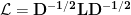
and non-diagonal components being zero. The following is the normalized Laplacian of the matrix L shown earlier.


Generally, we use only k eigenvalues to compute the graph distance. Thus, given two graphs G_1 and G_2, the spectral graph distance will be computed as

D(G_{1}, G_{2}) = \sqrt{\sum_{i=1}^{k} (\lambda_i^{g_1} - \lambda_i^{g_2})^2}

The spectral distance using adjacency matrix or any other matrix is computed similarly. 

Illustration of Spectral Graph Distance

Let’s now use the spectral graph distance on a small set of well-known graphs. We will compute the distance between different graph pairs to generate an inter-graph distance matrix. The following graphs are used.

  • American College Football
  • Les Miserables
  • Protein Network
  • Dolphins
  • Yeast
  • Celegans

These datasets were downloaded from network repository.com and the network data site. Three of these graphs, Football, Les Miserables, and Dolphins, are the social network graphs. The Protein Network and Yeast are biological graphs, and Celegans is a metabolic network.

I used the Netcomp package to do the distance computations. For no particular reason, I used the truncated spectra of 16 components. The inter-graph distance matrix and the resulting dendrogram using single link analysis are shown below. we can see that the spectral graph distance is able to cluster the social network graphs separately from the biological networks while the metabolic network, Celegans, is a cluster by itself.

The spectral graph distance is not the only method for computing distances between graphs; there are a few other methods as well. I hope to describe them in future posts.

Before you leave, please note that the spectral graph distance is not a metric. It doesn’t satisfy triangular inequality.

Understanding Loss Functions for Training Classifiers

Originally published on February 24, 2023

Building a classification model with a collection of annotated training examples requires making the following choices:

  • Classification model
    • This implies whether you should be using a logistic classifier or a multilayer neural network or a convolutional neural network or any other suitable model
  • Loss function
    • A loss function provides a measure of how well the training is proceeding and is needed to adjust the parameters of the classification model being trained. The choice of a loss function depends upon whether the model is being trained for a binary classification task or the number of classes is many.
  • Optimizer
    • The training involves optimizing the chosen loss function by repeatedly going over the training examples to adjust the model parameters. Again, there are several optimizers available in all popular machine learning and deep learning libraries to choose from.

In this blog post, I will focus on three commonly used loss functions for classification to give you a better understanding of these loss functions. These are:

  • Cross Entropy Loss
  • Binary Cross Entropy Loss
  • Negative Log-likelihood Loss

What is Cross Entropy?

Let’s first understand entropy which measures uncertainty of an event. We start by using C to represent a random event/variable which takes on different possible class labels as values in a training set. We use $p(c_i)$ to represent the probability that the class label of a training example is $c_i$, i.e. C equals $c_i$ with probability p. The entropy of the training set labels can be then expressed as below where the summation is carried over all possible labels:

$E(C) = -\sum_i p(c_i)$

It is easy to see that if all training examples are from the same class, then the entropy is zero, and there is no uncertainty about the class label of any training example picked at random. On the other hand, if the training set contains more than one class label, then we have some uncertainty about the class label of a randomly picked training example. As an example, suppose our training data has four labels: cat, dog, horse, and sheep. Let the mix of labels in our training data be cat 40%, dog 10%, horse 25%, and sheep 25%. Then the entropy of the training set using the natural log is given by

Entropy of our Training Set = -(0.4 log0.4 + 0.1log0.1 + 0.25log0.25 +   0.25log0.25 = 1.29

The entropy of a training set will achieve its maximum value when there are equal number of training examples from each category.

Let’s consider another random variable $\hat C$ which denotes the labels predicted by the model for a training example. Now, we have two sets of label distributions, one of true (target) labels in the training set and another of predicted labels. One way to compare these two label distributions is to extend the idea of entropy to cross entropy. It is defined as

$H(C,\hat{C}) = -\sum_i p(c_i)\log p(\hat{c}_i)$

Note that the cross entropy is not a symmetric function. Suppose the classifier that you have trained produces the following distribution of predicted labels: cat 30%, dog 15%, horse 25%, and sheep 30%. The cross entropy of the target and the predicted labels distribution is then given by

Cross Entropy(target labels, predicted labels) = -(0.4log0.3+ 0.1log0.15 + 0.25log0.25 +   0.25log0.3 = 1.32

The difference between the cross entropy value of 1.32 and the entropy of target labels of 1.29 is a measure of how close the predicted label distribution is to the target distribution.

While you are looking at your classifier, your friend pops in to tell you how well his classifier is doing. His classifier is producing the following distribution of predicted labels: cat 30%, dog 20%, horse 20%, and sheep 30%. You look at his numbers and tell him that your classifier is better that his because the cross entropy measure of your classifier, 1.32, is closer to the target entropy of 1.29 than the cross entropy measure of 1.35 of his classifier.

Cross Entropy Loss

The above definition of cross entropy is good for comparing two distributions or classifiers at a global level. However, we are interested in having a measure at the training examples level so that it can be used to adjust the parameters of the classifier being trained. To see how the above concept of cross entropy can be applied to each and every training example, let’s consider a training example inputted to a 3-class classifier to classify images of cats, dogs, and horses. The training example is of a horse. Using one-hot encoding for class labels, the target vector for the input image of the horse will be [0, 0, 1]. Since it is a 3-class problem, the classifier has three outputs as depicted below. where the output of the softmax stage is a vector of probabilities. Note that the classifier output is a vector of numbers, called logits. These are converted to a vector of probabilities by the softmax function as shown.


Thus, we have two sets of probabilities: one given by the target vector t and the second given by the output vector o. We can thus use the cross entropy measure defined earlier to express the cross entropy loss. Plugging in the numbers, the cross entropy loss value is calculated as

-(0*log(0.275) + 0*log(0.300) + 1*log(0.425)) -> 0.856

You can note that this loss would tend towards zero if the output probability for the class label horse goes up. This means that if our classifier is making correct predictions with increasing probabilities, the cross entropy loss will be small.

Since batches of training vectors are inputted at any training instance, the cross entropy loss for the batch is found by summing the loss over all examples.

While using the cross entropy loss in PyTorch, you do not need to worry about the softmax calculations. The cross entropy loss function in PyTorch takes logits as input and thus has a built-in softmax function. You can use the loss function for a single example or for a batch. The following example illustrates the use of cross entropy loss function for a single example.

import torch
import torch.nn.functional as F
out = torch.tensor([3.05, 3.13, 3.48])
target = torch.tensor([0.0, 0.0, 1.0])
loss =F.cross_entropy(out,target)
print(loss)
tensor(0.8566)

Binary Cross Entropy (BCE) Loss

Let’s consider a training model for a two-class problem. Let’s input an example from class 1 to the model, i.e the correct label is y = 1. The model predicts with probability p the input class label to be 1. The probability for the input class label not being 1 is then 1-p. The following formula captures the binary cross entropy loss for this situation:

$BCELoss = -(y*log(p) + (1-y)*log(1-p))$

Assuming p equal to 0.75, the BCELoss is 0.287. It is easy to see that when the predicted probability p approaches 1, the loss approaches 0.

loss = nn.BCELoss()
out= loss(torch.tensor([0.75]),torch.tensor([1.0]))
print(out)
tensor(0.2877)

The BCELoss function is generally used for binary classification problems. However, it can be used for multi-class problems as well. The BCELoss formula for C classes is then expressed as shown below where $y_k$ is the target vector component and $p_k$ is the predicted probability for class k.

$BCELoss = -\frac{1}{C}\sum_k (y_k * log(p_k) + (1-y_k)*log(1-p_k))$

Let’s use the above formula with a three-class problem where the predicted probabilities for an input for three classes are [0.277, 0.299, 0.424]. The training example is from class 3. The target tensor in this case is then [0.0,0.0,1.0]. The BCELoss value for this situation will be then

-(log(1-0.277) + log(1-0.299) + log(0.424))/3 –> 0.5125

We will now use the BCELoss function to validate our calculation.

out = loss(torch.tensor([0.277, 0.299, 0.424]), torch.tensor([0.0,0.0,1.0]))
print(out)
tensor(0.5125)

Note that the first argument in BCELoss() is a tensor of probabilities and the second argument is the target tensor. This means that the model should output probabilities. Often the output layer has the Relu function as the activation function. In such cases, Binary cross entropy with logits loss function should be used which converts the Relu output to probabilities before calculating the loss. This is shown below in the example where the first argument is a tensor of Relu output values. The calulations of the probabilities is also shown using the sigmoid function. You can use these probabilities in the BCELoss function to check whether you get the same loss value or not via these two different calculations.

loss = nn.BCEWithLogitsLoss()
out = loss(torch.tensor([1.8, 0.75]),torch.tensor([1.0,0.0]))
print (out)
print(torch.sigmoid(torch.tensor([1.8,0.75])))# Will output class probabilities
tensor(0.6449)
tensor([0.8581, 0.6792])

If we input the probabilities calculated above using the sigmoid function in the BCELoss function, we should get the same loss value.

loss = nn.BCELoss()
out= loss(torch.tensor([0.858,0.679]),torch.tensor([1.0, 0.0]))
print(out)
tensor(0.6447)

Negative Log Likelihood Loss

The negative log-likelihood loss (NLLLoss in PyTorch) is used for training classification models with C classes. The likelihood means what are the chances that a given set of training examples, $X_1,X_2,⋯,X_n$ was generated by a model that is characterized by a set of parameters represented by 𝜽. The likelihood 𝐿 thus can be expressed as 

$𝐿(X_1,X_2,⋯,X_n|\theta)=𝑃(X_1,X_2,⋯,X_n|\theta)$. 

Assuming that all training examples are independent of each other, the right hand side of the likelihood 𝐿 expression can be written as

$𝐿(X_1,X_2,⋯,X_n|\theta)= \prod(𝑃(X_1|\theta)𝑃(X_2|\theta)...𝑃(X_n|\theta)$.

Taking the log of the likelihood converts the right hand side multiplications to a summation. Since we are interested in minimizing the loss, the negative of the log likelihood is taken as the loss measure. Thus

$-log𝐿(X_1,X_2,⋯,X_n|\theta) = -\sum_{i=1}^{n}log(𝑃(X_i|\theta)$

The input to the NLLLoss function is log probabilities of each class as a tensor. The size of the input tensor is (minibatch size, C). The target specified in the loss is a class index in the range [0,C−1] where C = number of classes. Let’s take a look at an example of using NLLLoss function.

loss = nn.NLLLoss()
input = torch.tensor([[-0.6, -0.50, -0.30]])# minibatch size is 1 in this example. The log probabilities are all negative as expected.
target = torch.tensor([1])
output = loss(input,target)
print(output)
tensor(0.5000)

It can be noted that the NLLLoss value in this case is nothing but the negative of the log probability of the target class. When the class probabilities are not directly available as usually is the case, the model output needs to go through the LogSoftmax function to get log probabilities.

m = nn.LogSoftmax(dim=1)
loss = nn.NLLLoss()
# input is of size N x C. N=1, C=3 in the example
input = torch.tensor([[-0.8956, 1.1171, 1.3302]])
# each element in target has to have 0 <= value < C
target = torch.tensor([1])
output = loss(m(input), target)
print(output)
tensor(0.8634)

The cross entropy loss and the NLLLoss are mathematically equivalent. The difference between the two arises in how these two loss functions are implemented. As I mentioned earlier the cross entropy loss function in Pytorch expects logits as input, and it includes a softmax function while calculating the cross entropy loss. In the case of NLLLoss, the function expects log probabilities as input. Lacking them, we need to use LogSoftmax function to get the log probabilities as shown above.

There are a few other loss functions available in PyTorch and you can check them at the PyTorch documentation site. I hope you enjoyed reading my explanation of different loss functions. Contact me if you have any question.


Graph Classification using Graph Neural Networks

Graph classification focuses on assigning labels or categories to entire graphs or networks. Unlike traditional classification tasks that deal with individual data instances, graph classification considers the entire graph structure, including nodes, edges and their properties. A graph classifier uses a mapping function that can accurately predict the class or label of an unseen graph based on its structural properties. The mapping function is learned during training using supervised learning.

Why Do We Need Graph Classification?

The importance of graph classification lies in graph data being ubiquitous in today's interconnected world. Graph based methods including graph classification have emerged as methodology of  choice in numerous applications across various domains, including:

1. Bioinformatics: Classifying protein-protein interaction networks or gene regulatory networks can provide insights into disease mechanisms and aid in drug discovery. In fact, the most well-known success story of graph neural networks is the discovery of antibiotics to treat drug-resistant diseases, widely reported in early 2020.


2. Social Network Analysis: Categorizing social networks can help identify communities, detect anomalies (e.g., fake accounts), and understand information diffusion patterns.

3. Cybersecurity: Classifying computer networks can assist in detecting malicious activities, identifying vulnerabilities, and preventing cyber attacks.

4. Chemistry: Classifying molecular graphs can aid in predicting chemical properties, synthesizing new compounds, and understanding chemical reactions.

How Do We Build a Graph Classifier? 

There are two main approaches that we can use to build graph classifiers: kernel-based methods and neural network-based methods.

1. Kernel-based Methods:

These methods rely on defining similarity measures (kernels) between pairs of graphs, which capture their structural and topological properties. Popular kernel-based methods include the random walk kernel, the shortest-path kernel, and the Weisfeiler-Lehman kernel. Once the kernel is defined, traditional kernel-based machine learning algorithms, such as Support Vector Machines (SVMs), can be applied for classification.

2. Neural Network- based Methods:

These methods typically involve learning low-dimensional representations (embeddings) of the graphs through specialized neural network architectures, such as Graph Convolutional Networks (GCNs) and Graph Attention Networks (GATs). The learned embeddings capture the structural information of the graphs and can be used as input to standard classifiers, like feed-forward neural networks or logistic regression models. For details on GCNs and node embeddings, please visit my earlier post on graph convolutional networks

Both kernel-based and neural network-based methods have their strengths and weaknesses, and the choice depends on factors such as the size and complexity of the graphs, the availability of labeled data, and computational resources. Given that graph neural networks are getting more mileage, we will complete this blog post by going over steps needed for building a GNN classifier.

Steps for Building a GNN Classifier

Dataset

We are going to use the MUTAG dataset which is part of the TUDatasets, an extensive collection of graph datasets and easily accessible in PyTorch Geometric library for building graph applications. The MUTAG dataset is a small dataset of 188 graphs representing two classes of graphs. Each graph node is characterized by seven features. Two of the example graphs from this dataset are shown below.

Two example graphs from MUTAG dataset


We will use 150 graphs for training and the remaining 38 for testing. The division into the training and test sets is done using the available utilities in the PyTorch Geometric. 

Mini-Batching

Due to the smaller graph sizes in the dataset, mini-batching of graphs is a desirable step in graph classification for better utilization of GPU resources. The mini-batching is done by diagonally stacking adjacency matrices of the graphs in a batch to create a giant graph that acts as an input to the GNN for learning. The node features of the graphs are concatenated to form the corresponding giant node feature vector. The idea of mini-batching is illustrated below.


Illustration of mini-batching


Graph Classifier

We are going to use a three-stage classifier for this task. The first stage will consists of generating node embeddings using a message-passing graph convolutional network (GCN). The second stage is an embeddings aggregation stage. This stage is also known as the readout layer. The function of this stage is to aggregate node embeddings into a single vector. We will simply take the average of node embeddings to create readout vectors. PyTorch Geometric has a built-in function for this purpose operating at the mini-batch level that we will use. The final stage is the actual classifier that looks at mapped/readout vectors to learn classification rule. In the present case, we will simply use a linear thresholding classifier to perform binary classification. We need to specify a suitable loss function so that the network can be trained to learn the proper weights.

A complete implementation of all of the steps described above is available at this Colab notebook. The results show that training a GCN with three convolutional layers results in test accuracy of 76% in just a few epochs.

Takeaways Before You Leave

Graph Neural Networks (GNNs) offer ways to perform various graph-related prediction/classification tasks. We can use GNNs make predictions about nodes, for example designate a node as a friend or fraud. We can use them to predict whether a link should exist between a pair of nodes or not in social networks to make friends' suggestions. And of course, we can use GNNs to perform classification of entire graphs with applications mentioned earlier.

Another useful library for deep learning with graphs is Deep Graph Library (DGL). You can find a graph classifier implementation using DGL at the following link, if you like.