Graph-based representation is a natural choice in many areas such as biology, computer science, communication, social sciences, and telecommunication. Such representations are also known as network models. Often, we are interested in finding out how much different the two graphs are and want to specify that difference in the form of a numerical measure such as the distance or similarity between a pair of graphs. Measuring the distance between two graphs is different from the graph isomorphism problem where we look for a mapping based on one-to-one correspondence between the nodes of the two graphs. In this blog post, I am going to describe the graph distance measure, spectral graph distance, which has been suggested and used to measure the difference between a pair of graphs. In the subsequent blog posts, I intend to describe some other graph distance/similarity measures.
Graph Basics
Before describing the spectral graph distance, let’s take a look at some basic definitions related to graphs. A graph is represented as G(V, E) where V represents a list of vertices/nodes and E represents a list of edges between those nodes. The adjacency matrix A of a graph is matrix of size |V|x|V| where |V| is the number of vertices or nodes in the graph. The element $a_{ij}$ of the adjacency matrix is 1 if there is an edge between the vertex-i and vertex-j; otherwise it is 0. This is true for undirected graphs without weights assigned to edges. An example of a graph G and its adjacency matrix are shown below.
 |
| An example graph with its adjacency matrix |

Another matrix of interest is the Laplacian matrix of a graph. It is defined as L = D – A. The Laplacian matrix is known to capture many useful properties of a graph. The Laplacian matrix of an undirected graph is a symmetric matrix and so is the adjacency matrix. The Laplacian matrix for the above example graph is given as

Spectral Graph Distance
The eigenvalues of the graph matrices, adjacency or Laplacian, provide information about the graph’s structural properties, such as the number of connected components, the density of the graph, and the distribution of degrees. Thus, comparing two sets of eigenvalues coming from two different graphs, we can compute the distance between them. Such a distance measure then can be used for various graphs related tasks, for example for clustering graphs or monitoring changes in a graph over time. The comparison between the two sets of eigenvalues is done by sorting the respective eigenvalues in descending (for adjacency matrices) or ascending (for Laplacian matrices) order. The sorted eigenvalues of a matrix define its spectrum. For example, the spectrum of the above adjacency matrix is 3.323 ≥ 0.357 ≥ -1 ≥ -1 ≥ -1.681, while the Laplacian matrix spectrum is 0 ≤ 2 ≤ 4 ≤ 5 ≤ 5.
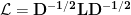
The Laplacian matrix is preferred for calculating the spectral graph distance because of its properties. The Laplacian matrix of an undirected graph is a positive-semidefinite matrix and thus its eigenvalues are all positive. Further, the sum of every row or column is 0 and thus the smallest eigenvalue is always 0. The number of eigenvalues equal to 0 indicates the number of connected components in the graph. It turns out that the presence of a vertex with a high degree of connectivity tends to dominate the Laplacian matrix. To avoid this, it is common to normalize the Laplacian matrix. The normalized Laplacian matrix is defined as
where the diagonal components of the matrix 


Generally, we use only k eigenvalues to compute the graph distance. Thus, given two graphs 


The spectral distance using adjacency matrix or any other matrix is computed similarly.
Illustration of Spectral Graph Distance
Let’s now use the spectral graph distance on a small set of well-known graphs. We will compute the distance between different graph pairs to generate an inter-graph distance matrix. The following graphs are used.
- American College Football
- Les Miserables
- Protein Network
- Dolphins
- Yeast
- Celegans
These datasets were downloaded from network repository.com and the network data site. Three of these graphs, Football, Les Miserables, and Dolphins, are the social network graphs. The Protein Network and Yeast are biological graphs, and Celegans is a metabolic network.
I used the Netcomp package to do the distance computations. For no particular reason, I used the truncated spectra of 16 components. The inter-graph distance matrix and the resulting dendrogram using single link analysis are shown below. we can see that the spectral graph distance is able to cluster the social network graphs separately from the biological networks while the metabolic network, Celegans, is a cluster by itself.

The spectral graph distance is not the only method for computing distances between graphs; there are a few other methods as well. I hope to describe them in future posts.
Before you leave, please note that the spectral graph distance is not a metric. It doesn’t satisfy triangular inequality.
