CountVectorizer to HashingVectorizer for Numeric Representation of Text

According to some estimates, the unstructured data accounts for about 90% of the data being generated everyday. A large part of unstructured data consists of text in the form of emails, news reports, social media postings, phone transcripts, product reviews etc. Analyzing such data for pattern discovery requires converting text to numeric representation in the form of a vector using words as features. Such a representation is known as vector space model in information retrieval; in machine learning it is known as bag-of-words (BoW) model.

In this post, I will describe different text vectorizers from sklearn library. I will do this using a small corpus of four documents, shown below.

corpus = ['The sky is blue and beautiful',
'The king is old and the queen is beautiful',
'Love this beautiful blue sky',
'The beautiful queen and the old king']

CountVectorizer

The CountVectorizer is the simplest way of converting text to vector. It tokenizes the documents to build a vocabulary of the words present in the corpus and counts how often each word from the vocabulary is present in each and every document in the corpus. Thus, every document is represented by a vector whose size equals the vocabulary size and entries in the vector for a particular document show the count for words in that document. When the document vectors are arranged as rows, the resulting matrix is called document-term matrix; it is a convenient way of representing a small corpus.

For our example corpus, the CountVectorizer produces the following representation.

from sklearn.feature_extraction.text import CountVectorizer
import pandas as pd
vectorizer = CountVectorizer()
X = vectorizer.fit_transform(corpus)
print(vectorizer.get_feature_names())
Doc_Term_Matrix = pd.DataFrame(X.toarray(),columns= vectorizer.get_feature_names())
Doc_Term_Matrix

['and', 'beautiful', 'blue', 'is', 'king', 'love', 'old', 'queen', 'sky', 'the', 'this']

The column headings are the word features arranged in alphabetical order and row indices refer to documents in the corpus. In the present example, the size of the resulting document-term matrix is 4×11, as there are 4 documents in the example corpus and there are 11 distinct words in the corpus. Since common words such as “is”, “the”, “this” etc do not provide any indication about the document content, we can safely remove such words by telling CountVectorizer to perform stop word filtering as shown below.

vectorizer = CountVectorizer(stop_words='english')
X = vectorizer.fit_transform(corpus)
print(vectorizer.get_feature_names())
Doc_Term_Matrix = pd.DataFrame(X.toarray(),columns= vectorizer.get_feature_names())
Doc_Term_Matrix

['beautiful', 'blue', 'king', 'love', 'old', 'queen', 'sky']

Although the document-term matrix for our small corpus example doesn’t have too many zeros, it is easy to conceive that for any large corpus the resulting matrix will be a sparse matrix. Thus, internally the sparse matrix representation is used to store document vectors.

N-gram Word Features

One issue with the bag of words representation is the loss of context. The BoW representation just focuses on words presence in isolation; it doesn’t use the neighboring words to build a more meaningful representation. The CountVectorizer provides a way to overcome this issue by allowing a vector representation using N-grams of words. In such a model, N successive words are used as features. Thus, in a bi-gram model, N = 2, two successive words will be used as features in the vector representations of documents. The result of such a vectorization for our small corpus example is shown below. Here the parameter ngram_range = (1,2) tells the vectorizer to use two successive words along with each single word as features for the resulting vector representation.

vectorizer = CountVectorizer(ngram_range = (1,2),stop_words='english')
X = vectorizer.fit_transform(corpus)
print(vectorizer.get_feature_names())
Doc_Term_Matrix = pd.DataFrame(X.toarray(),columns= vectorizer.get_feature_names())
Doc_Term_Matrix

['beautiful', 'beautiful blue', 'beautiful queen', 'blue', 'blue beautiful', 'blue sky', 'king', 'king old', 'love', 'love beautiful', 'old', 'old king', 'old queen', 'queen', 'queen beautiful', 'queen old', 'sky', 'sky blue']

It is obvious that while N-gram features provide context and consequently better results in pattern discovery, it comes at the cost of increased vector size.

TfidfVectorizer

Simply using the word count as a feature value of a word really doesn’t reflect the importance of that word in a document. For example, if a word is present frequently in all documents in a corpus, then its count value in different documents is not helpful in discriminating between different documents. On other hand, if a word is present only in a few of documents, then its count value in those documents can help discriminating them from the rest of the documents. Thus, the importance of a word, i.e. its feature value, for a document not only depends upon how often it is present in that document but also how is its overall presence in the corpus. This notion of importance of a word in a document is captured by a scheme, known as the term frequency-inverse document frequency (tf-idf ) weighting scheme.

The term frequency is a ratio of the count of a word’s occurrence in a document and the number of words in the document. Thus, it is a normalized measure that takes into consideration the document length. Let us show the count of word i in document j by . The document frequency of word i represents the number of documents in the corpus with word i in them. Let us represent document frequency for word i by . With N as the number of documents in the corpus, the tf-idf weight for word i in document j is computed by the following formula:

The sklearn library offers two ways to generate the tf-idf representations of documents. The TfidfTransformer transforms the count values produced by the CountVectorizer to tf-idf weights.

from sklearn.feature_extraction.text import TfidfTransformer
transformer = TfidfTransformer()
tfidf = transformer.fit_transform(X)
Doc_Term_Matrix = pd.DataFrame(tfidf.toarray(),columns= vectorizer.get_feature_names())
pd.set_option("display.precision", 2)
Doc_Term_Matrix

Another way is to use the TfidfVectorizer which combines both counting and term weighting in a single class as shown below.

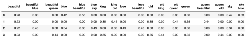
from sklearn.feature_extraction.text import TfidfVectorizer
vectorizer = TfidfVectorizer(ngram_range = (1,2),stop_words='english')
tfidf = vectorizer.fit_transform(corpus)
Doc_Term_Matrix = pd.DataFrame(tfidf.toarray(),columns= vectorizer.get_feature_names())
Doc_Term_Matrix

One thing to note is that the tf-idf weights are normalized so that the resulting document vector is of unit length. You can easily check this by squaring and adding the weight values along each row of the document-term matrix; the resulting sum should be one. This sum represents the squared length of the document vector.

HashingVectorizer

There are two main issues with the CountVectorizer and TdidfVectorizer. First, the vocabulary size can grow so much so as not to fit in the available memory for large corpus. In such a case, we need two passes over data. If we were to distribute the vectorization task to several computers, then we will need to synchronize vocabulary building across computing nodes. The other issue arises in the context of an online text classifier built using the count vectorizer, for example spam classifier which needs to decide whether an incoming email is spam or not. When such a classifier encounters words not in its vocabulary, it ignores them. A spammer can take advantage of this by deliberately misspelling words in its message which when ignored by the spam filter will cause the spam message appear normal.  The HashingVectorizer overcomes these limitations.

The HashingVectorizer is based on feature hashing, also known as the hashing trick. Unlike the CountVectorizer where the index assigned to a word in the document vector is determined by the alphabetical order of the word in the vocabulary, the HashingVectorizer maintains no vocabulary and determines the index of a word in an array of fixed size via hashing. Since no vocabulary is maintained, the presence of new or misspelled words doesn’t create any problem. Also the hashing is done on the fly and memory need is diminshed.

You may recall that hashing is a way of converting a key into an address of a table, known as the hash table. As an example, consider the following hash function for a string s of length n:

$\text{hash(s)} = (s[0] + s[1] \cdot p +s[2]\cdot p^2 +\cdots  + s[n-1] \cdot p^{n-1})\text{ mod }m$

The quantities p and m are chosen in practice to minimize collision and set the hash table size. Letting p = 31 and m = 1063, both prime numbers, the above hash function will map the word “blue” to location 493 in an array of size 1064 as per the calculations:

where letter b is replaced by 2, l by 12, and so on based on their positions in the alphabet sequence. Similarly, the word “king” will be hashed to location 114 although “king” comes later than “blue” in alphabetical order.

The HashingVectorizer implemented in sklearn uses the  Murmur3 hashing function which returns both positive and negative values. The sign of the hashed value is used as the sign of the value stored in the document-term matrix. By default, the size of the hash table is set to ; however, you can specify the size if the corpus is not exceedingly large. The result of applying HashingVectorizer to our example corpus is shown below. You will note that the parameter n_features, which determines the hash table size, is set to 6. This has been done to show collisions since our corpus has 7 distinct words after filtering stop words.

from sklearn.feature_extraction.text import HashingVectorizer
vectorizer = HashingVectorizer(n_features=6,norm = None,stop_words='english')
X = vectorizer.fit_transform(corpus)
Doc_Term_Matrix = pd.DataFrame(X.toarray())
Doc_Term_Matrix

You will note that column headings are integer numbers referring to hash table locations. Also that hash table location indexed 5 shows the presence of collisions. There are three words that are being hashed to this location. These collisions disappear when the hash table size is set to 8 which is more than the vocabulary size of 7. In this case, we get the following document-term matrix.

The HashingVectorizer has a norm parameter that determines whether any normalization of the resulting vectors will be done or not. When norm is set to None as done in the above, the resulting vectors are not normalized and the vector entries, i.e. feature values, are all positive or negative integers. When norm parameter is set to l1, the feature values are normalized so as the sum of all feature values for any document sums to positive/negative 1. In the case of our example corpus, the result of using l1 norm will be as follows.

With norm set to l2, the HashingVectorizer normalizes each document vector to unit length. With this setting, we will get the following document-term matrix for our example corpus.

The HashingVectorizer is not without its drawbacks. First of all, you cannot recover feature words from the hashed values and thus tf-idf weighting cannot be applied. However, the inverse-document frequency part of the tf-idf weighting can be still applied to the resulting hashed vectors, if needed. The second issue is that of collision. To avoid collisions, hash table size should be selected carefully. For very large corpora, the hash table size of or more seems to give good performance. While this size might appear large, some comparative numbers illuminate the advantage of feature hashing. For example, an email classifier with hash table of size 4 million locations has been shown to perform well on a well-known spam filtering dataset having 40 million unique words extracted from 3.2 million emails. That is a ten times reduction in the document vectors size.

To summarize different vectorizers, the TfidfVectorizer appears a good choice and possibly the most popular choice for working with a static corpus or even with a slowing changing corpus provided periodic updating of the vocabulary and the classification model is not problematic. On the other hand, the HashingVectorizer is the best choice when working with a dynamic corpus or in an online setting.

Embeddings Beyond Words: Intro to Sentence Embeddings

It wouldn't be an exaggeration to say that the recent advances in Natural Language Processing (NLP) technology can be, to a large extent, attributed to the use of very high-dimensional vectors for language representation. These high-dimensional, 764 dimensions is common, vector representations are called embeddings and are aimed at capturing semantic meaning and relationships between linguistic items.

Although the idea of using vector representation for words has been around for many years, the interest in word embedding took a quantum jump with Tomáš Mikolov’s Word2vec algorithm in 2013. Since then, many methods for generating word embeddings, for example GloVe and BERT, have been developed. Before moving on further, let's see briefly how word embedding methods work.

Word Embedding: How is it Performed?

I am going to explain how word embedding is done using the Word2vec method. This method uses a linear encoder-decoder network with a single hidden layer. The input layer of the encoder is set to have as many neurons as there are words in the vocabulary for training. The hidden layer size is set to the dimensionality of the resulting word vectors. The size of the output layer is same as the input layer. The input words to the encoder are encoded using one-hot vector encoding where the size of the vector corresponds to the vocabulary. The figure below shows the arrangement for learning embeddings.

The embeddings are learned by adjusting weights so that for a target word, say fox in a piece of text "The quick brown fox jumped over the fence", the probability for the designated context word, say jumped is high. There are two major variations to this basic technique. In a variation known as the continuous bag of words (CBW), multiple context words are used. Thus, the system may use brown, jumped and fence as the context words. In another scheme, known as the skip-gram model, the use of target and context words is reversed. Thus, the target word is fed on the input side and the weights are modified to increase probabilities for the prediction of context words. In both of these cases, the above architecture needs modification. You can read details about the architecture changes as well as look at a simple example in the blog post that I did a while ago.

Sentence Embeddings

While word embeddings are useful, we are often working with text to perform tasks such as text classification, sentiment analysis, and topic detection etc. Thus, it would be logical to extend the idea of word embeddings to sentences.  One simple way to accomplish this is to take the average of embeddings of different words in a sentence. However, such an approach doesn't take into account the word order and thus results in vectors that aren't very good at capturing the sentence meaning. Instead, the sentence embeddings are obtained by using transformer models such BERT (Bidirectional Encoder Representations from Transformers) which make use of attention mechanism to gauge the importance of different words in a sentence. BERT outputs for each token in the given input text its contextualized embedding. In order to create a fixed-sized sentence embedding out of this, the model applies mean pooling, i.e., the output embeddings for all tokens are pooled to yield a fixed-sized vector. The Sentence-BERT or simply SBERT is a package that you can use to create sentence embeddings without worrying about pooling. 

One issue facing BERT/SBERT is that of encountering an out of vocabulary word, that is a word that wasn't part of the text corpus used to train BERT. In such a case, an embedding for such a word doesn't exist. BERT/SBERT solve this by using a WordPiece tokenizer which breaks every word into one or more tokens. As an example, the word snowboarding will be tokenized through three tokens: snow, board, ing. This ensures embedding being created for any new word. SBERT permits creating a single vector embedding for sequences containing no more than 128 tokens. Sequence tokens beyond 128 are simply discarded.

Sentence Embedding Libraries

Other than SBERT, there are many libraries that one can use. Some of these are:

• TensorFlow Hub - Provides pre-trained encoders like BERT and other transformer models. Makes it easy to generate sentence embeddings.

• InferSent - Facebook AI research model for sentence embeddings trained on natural language inference data.

• Universal Sentence Encoder (USE) - Google model trained on a variety of data sources to generate general purpose sentence embeddings.

• Flair - NLP library with models like Flair embeddings trained on unlabeled data which can provide sentence representations.

• Doc2Vec - Extension of Word2Vec that can learn embeddings for sentences and documents.

• Stanford SkipThoughts - Unupervised model trained to predict surrounding sentences based on context.

• GenSim - Includes implementations of models like Doc2Vec for generating sentence and paragraph embeddings.

• SentenceTransformers - Library for state-of-the-art sentence embeddings based on transformers. Includes pretrained models like BERT and RoBERTa.

The choice of model depends on your use case. For general purposes, pretrained universal encoders like USE and SBERT provide robust sentence vectors. For domain-specific tasks, fine-tuning transformer models like BERT often produces the best performance.

One word of caution while using embeddings. Never mix embeddings generated by two different libraries. Embeddings produced via each method/framework are unique to that method and the training corpus.

An Example of Sentence Embedding for Measuring Similarity

Let's take a look at using sentence embedding to capture semantic similarity between pairs of sentences. We will use SBERT for this purpose. First, we install and import the necessary libraries and decide upon the sentence transformer model to be used.

! pip install sentence-transformers




from sentence_transformers import SentenceTransformer

model = SentenceTransformer('all-mpnet-base-v2')

Next, we specify the sentences that we are using.

sentences = [

"The sky is blue and beautiful",

"Love this blue and beautiful sky!",

"The brown fox is quick and the blue dog is lazy!",

"The dog is lazy but the brown fox is quick!",

"the bees decided to have a mutiny against their queen",

"the sign said there was road work ahead so she decided to speed up",

"on a scale of one to ten, what's your favorite flavor of color?",

"flying stinging insects rebelled in opposition to the matriarch"

]

embeddings = model.encode(sentences)

embeddings.shape

(8, 768)

So, the embedding results in eight vectors of 768 dimensions. Next, we import a utility from sentence transformer library and compute cosine similarities between different pairs. Remember, the cosine similarity value close to one indicates very high degree of similarity and low values are indicative of almost no similarity.

from sentence_transformers import util
#Compute cosine similarity between all pairs
cos_sim = util.cos_sim(embeddings, embeddings)
print(cos_sim)

tensor([[ 1.0000, 0.7390, 0.2219, 0.1689, 0.1008, 0.1191, 0.2174, 0.0628], [ 0.7390, 1.0000, 0.1614, 0.1152, 0.0218, 0.0713, 0.2854, -0.0181], [ 0.2219, 0.1614, 1.0000, 0.9254, 0.1245, 0.2171, 0.1068, 0.0962], [ 0.1689, 0.1152, 0.9254, 1.0000, 0.1018, 0.2463, 0.0463, 0.0706], [ 0.1008, 0.0218, 0.1245, 0.1018, 1.0000, 0.2005, 0.0153, 0.6084], [ 0.1191, 0.0713, 0.2171, 0.2463, 0.2005, 1.0000, 0.0116, 0.1011], [ 0.2174, 0.2854, 0.1068, 0.0463, 0.0153, 0.0116, 1.0000, -0.0492], [ 0.0628, -0.0181, 0.0962, 0.0706, 0.6084, 0.1011, -0.0492, 1.0000]])

Looking at the resulting similarity values, we see that the sentence#1 and sentence#2 pair has a high degree of similarity. Sentence#3 and sentence#4 also generate a very high value of cosine similarity. Interestingly, sentence#5 and sentence#8 are also deemed to have a good semantic similarity, although they do not share any descriptive words. Thus, the sentence embedding is doing a pretty good job of capturing sentence semantics.

Comparison with TF-IDF Vectorization

Information Retrieval (IR) community for a long time has been representing text as vectors for matching documents. The approach, known as the bag-of-words model, uses a set of words or terms to characterize text.  Each word or term is assigned a weight following the  TF-IDF weighting scheme. In this scheme, the weight assigned to a word is based upon: (i) how often it appears in the document being vectorized, the term frequency (TF) component of the weighting scheme, and (ii) how rare is the word in the entire document collection, the inverse document frequency (IDF) component of the weighting scheme. The vector size is governed by the number of terms used from the entire document collection, i.e. the vocabulary size. You can read details about TF-IDF vectorization in this blog post.

Let's see how well the TF-IDF vectorization captures similarities between document in comparison with the sentence embedding. We will use the same set of sentences to perform vectorization and similarity calculations as shown below.

from sklearn.feature_extraction.text import TfidfVectorizer

from sklearn.metrics.pairwise import cosine_similarity

vectorizer = TfidfVectorizer(ngram_range = (1,2),stop_words='english')

tfidf = vectorizer.fit_transform(sentences)

similarity =cosine_similarity(tfidf,tfidf)

np.set_printoptions(precision=4)

print(similarity)

[[1. 0.5818 0.0962 0. 0. 0. 0. 0. ] [0.5818 1. 0.0772 0. 0. 0. 0. 0. ] [0.0962 0.0772 1. 0.7654 0. 0. 0. 0. ] [0. 0. 0.7654 1. 0. 0. 0. 0. ] [0. 0. 0. 0. 1. 0.0761 0. 0. ] [0. 0. 0. 0. 0.0761 1. 0. 0. ] [0. 0. 0. 0. 0. 0. 1. 0. ] [0. 0. 0. 0. 0. 0. 0. 1. ]]

Looking at the above results, we see that TF-IDF vectorization is unable to determine similarity between 
sentence#5 and sentence#8 which the sentence embedding was able to pick up despite of the absence of the common descriptive words in the sentence pair.

Thus, TF-IDF vectorizer is good as long as there are shared descriptive words. But the sentence embedding is able to capture semantic similarities without even shared descriptive words. This is possible because the high-dimensional embedded vectors learn relationships between different words and their context during training and utilize those relationships during similarity computation as well as for other NLP tasks.

Now you might be wondering whether the embedding concept can be applied to images and graphs. The answer is yes and I hope to dwell on these in my future posts.