LLaMA 2 and its Symbolic Regression Explanation

On July 17, a new family of AI models, LLaMA 2 was announced by Meta. LLaMA 2 is trained on a mix of publicly available data. According to Meta LLaMA 2 performs significantly better than the previous generation of LLaMA models. Two flavors of the model: LLaMA 2 and LLaMA 2-Chat, a model fine tuned for two-way conversations, were released. Each flavor further has three versions with the parameters ranging from 7 billions to 70 billions. Meta is also freely releasing the code and data behind the model for  researchers to build upon and improve the technology.

There are several ways to access LLaMA 2 for development work; you can download it from HuggingFace or access it via Microsoft Azure or Amazon SageMaker. For those interested in interacting with the LLaMA 2-Chat version, you can do so by visiting llama2.ai, a chatbot model demo hosted by the venture capitalist Andreessen Horowitz. This is the route I took to interact with LLaMA 2-Chat.

Since I was reading an excellent paper on symbolic regression, I decided to query LLaMA 2-Chat about this topic. Before I show my chat with the model, let me explain symbolic regression if you are not familiar with it. In the traditional linear regression, the model form, linear or polynomial etc., is assumed and the coefficients/parameters of the model are determined to get the best possible accuracy. In contrast, the symbolic regression involves searching a space of analytical expressions with the corresponding parameter values to best model a given dataset. 

I started off by asking if LLaMA-2 Chat is better than GPT-4. I followed it up by asking about symbolic regression as shown below. 


The answer provided was not specific. So I asked LLaMA 2 for a concrete example. This resulted in the conversation shown below.

Clearly, the example provided is that of linear regression and not of symbolic regression. Pointing this out to LLaMA 2 resulted in the following conversation, where again I had to point out that symbolic regression searching for different functions.


As you can see, LLaMA 2 had difficulty explaining symbolic regression and needed to be prompted for making mistakes. Next, I decided to go to ChatGPT to see what kind of response it would produce. Below is the ChatGPT output.


As you can see, ChatGPT was clear in explaining symbolic regression and even mentioned about the use of genetic algorithms and genetic programming that are key to symbolic regression.


So my take is to stick with Chat-GPT for getting help on topics of interest. LLaMA 2 is lacking in providing clear explanations. Of course, my take is based only on conversation about one topic only.


Low Rank Adaptation (LoRA): Enhancing Fine-Tuning of LLMs

Pre-trained large language models (LLMs) are being used for numerous natural language processing applications. These models perform well out of the box and are fine-tuned for any desired down-stream application. However, fine-tuning these models to adapt to specific tasks often poses challenges due to their large parameter sizes. To address this, a technique called Low Rank Adaptation (LoRA) has emerged, enabling efficient fine-tuning of LLMs. In this post, we will try to understand LoRA, and delve into its importance and application in fine-tuning LLMs. We will begin our journey by first looking at the concept of rank of a matrix, followed by a look at matrix factorization, and then to LoRA.

Rank of a Matrix

The rank of a matrix indicates the number of independent rows or column in the matrix. As an example, consider the following 4x4 matrix A:

A = [[2, 4, 6, 8], [1, 3, 5, 7], [4, 8, 12, 16], [3, 9, 15, 21]]

Looking at the first and third row of this matrix, we see that the third row is just a scale up version of the first row by a factor of 2. The same is true for the second and fourth rows. Thus, the rank of matrix A is 2 as there are only two independent rows. 

The rank of a matrix of size mxn cannot be greater than min{m,n}. In other words, the rank of a matrix cannot be greater than the smallest dimension of the matrix. We say a matrix is a full rank matrix if its rank equals the largest possible rank for that matrix. 

When a matrix is not a full rank matrix, it tells us that the underlying matrix has some redundancy in it that can be exploited for data compression or dimensionality reduction. This is done by obtaining a low-rank approximation of the matrix. The process of obtaining a low-rank approximation of a matrix is involves matrix factorization. Some of these factorization methods are briefly described below. 

Matrix Factorization

Matrix factorization is the process of decomposing a matrix into multiple factors. Some of the matrix factorization are:

1. Singular Value Decomposition (SVD)

In SVD, a real-valued matrix A of size m x n is factorized as $ A =  UDV^t$, where 𝐔 is an orthogonal matrix of size m x m of left singular vectors and 𝐕 is an orthogonal matrix of size n x n of right singular vectors. The matrix 𝐃 is a diagonal matrix of size m x n of singular values. A low rank approximation to matrix A of rank r is obtained by using only a subset of singular values and the corresponding left and right singular vectors as given by the following expression. In other words, the approximation is obtained by the weighted sum of rank one matrices.
$ \hat{ \bf A} = \sum\limits_{j=1}\limits^{k} d_{jj}\bf U_j\bf V^t,\text{   }k\leq r$

SVD is a popular matrix factorization method that is commonly used for data compression and dimensionality reduction. It has also been used for compressing convolutional neural networks. You can read more about SVD and its use for compression at this blog post.

2. Principal Component Analysis (PCA)

PCA aims to find the principal components that capture the most significant variance in the data. It works with data matrices that have been normalized to have zero mean. Let's say $X$ of m rows and n columns is one such data matrix where each row represents an observation vector of n features. PCA computes the eigenvalues and eigenvectors of the covariance matrix $C = \frac{1}{(1-n)}XX^t$ by factorizing it as $\frac{1}{(1-n)}WD^tW$, where $W$ is an orthogonal matrix of eigenvectors and $D$ is the diagonal matrix of eigenvalues. PCA is a popular technique for dimensionality reduction.

3. Non-Negative Matrix Factorization (NMF)

NMF is another technique for obtaining low rank representation of matrices with non-negative or positive elements. Given a data matrix $A$ of m rows and n columns with each and every element $a_{ij} ≥ 0$, NMF seeks matrices $W$ and $H$ of size m rows and k columns, and k rows and n columns, respectively, such that $A≈WH$, and every element of matrices $W$ and $H$ is either zero or positive. The value of k is set by the user and is required to be equal or less than the smallest of m and n. The matrix $W$  is generally called the basis matrix, and $H$ is known as expansion or coefficient matrix. The underlying idea of this terminology is that a given data matrix $A$ can be expressed in terms of summation of k basis vectors (columns of $W$) multiplied by the corresponding coefficients (columns of $H$). Compared to SVD, the NMF based factorization offers a better interpretation of the original data matrix as it is represented/approximated as a sum of positive matrices/vectors. NMF has been used to perform document clustering, making recommendations, visual pattern recognition such as face recognition, gene expression analysis, feature extraction, source separation etc. Basically, it can be used in any application where data matrix $A$ has no negative elements. You can read more about NMF at this blog post.


Low Rank Adaptation (LoRA) of Large Language Models

The first thing to note is that LoRA doesn't perform a low rank approximation of the weight or parameter matrix; it rather modifies it by generating a new low rank matrix that captures the needed parameter changes as a result of the fine tuning the LLM. The pre-trained matrix $W$ is frozen while fine tuning and the weight changes are captured in a delta weight matrix $\Delta W$ through gradient learning. The delta weight change matrix is a low rank matrix which is set as a product of two small matrices, i.e. $\Delta W = AB$. The $A$ matrix is initialized with values coming from a gaussian distribution while $B$ matrix is initialized with elements all equal to zero. This ensures that the pre-trained weights matrix is the only contributing matrix at the start of fine tuning. The figure below illustrates this setup for LoRA.


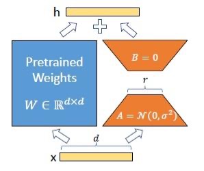
LoRA Scheme: Matrix W is kept fixed and only A and B are trained.

Let's now try to understand the reasoning behind LoRA and its advantages. The main motivation is that the pretrained models are over-parameterized with low intrinsic dimensionality. Further, the authors of LoRA hypothesize that change in weights during model fine tuning also has a low intrinsic rank. Thus, it is suffice to use a low rank matrix to capture the weight changes during fine tuning. LoRA offers several advantages. First, it is possible to share the pretrained model for several downstream tasks with each task having its own LoRA model. This obviously saves storage needs as well as makes task switching easier. Second, LoRA makes the LLMs adaptation for different tasks easier and efficient. Third, it is easy to combine with other fine tuning methods, if desired. As an example of the parameter efficiency of LoRA, consider the pretrained matrix of size 200x400. To perform adaptation, let matrix $A$ be of size 200x8 and matrix $B$ be of size 8x400 giving rise to the delta weight change matrix of the desired size of 200x400. The number of parameters thus needed by LoRA is only 200*8+8*400 = 4800 as compared to the number of parameter, 200*400 = 80000, needed to adjust without LoRA.

An important consideration in using LoRA is the choice of the rank of the $\Delta W$ matrix. Choosing a smaller rank leads to a simpler low-rank matrix, which results in fewer parameters to learn during adaptation. However, the adaptation with a smaller rank $\Delta W$ may not lead to the desired performance. Thus, the rank choice offers a tradeoff that typically requires experimentation to get the best adaptation. 

LoRA in PEFT

PEFT stands for a general parameter-efficient fine-tuning library from Huggins Face that includes LoRA as one of its techniques. The few lines of codes below illustrate its basic use.


from transformers import AutoModelForSeq2SeqLM
from peft import get_peft_config, get_peft_model, LoraConfig, TaskType
model_name_or_path = "bigscience/mt0-large"
tokenizer_name_or_path = "bigscience/mt0-large"

peft_config = LoraConfig(
    task_type=TaskType.SEQ_2_SEQ_LM, inference_mode=False, r=8, lora_alpha=32, lora_dropout=0.1
)

model = AutoModelForSeq2SeqLM.from_pretrained(model_name_or_path)
model = get_peft_model(model, peft_config)
model.print_trainable_parameters()
# output: trainable params: 2359296 || all params: 1231940608 || trainable%: 0.19151053100118282


In the above example, mt0-large model is being fine tuned for a sequence to sequence conversion task. The rank of the delta weight change is specified as 8.  The model has 1.2 B parameters but LoRA needs only 2.36M parameters, 19% of the total parameters, to train. If we are to change the rank to 12, the number of trainable parameters increases to 3538944, 28.7% of the total parameters. Clearly, the choice of rank is an important consideration when using LoRA.

LoRA's performance has been evaluated against full fine tuning and other efficient techniques for parameter computation. LoRA has been found to generally outperforms other efficient fine tuning techniques by a significant margin while yielding comparable or better performance than full fine tuning. 

To wrap up, LoRA is an efficient technique for fine tuning large pretrained models. It is poised to play an important role in fine tuning and customizing LLMs for numerous applications.

It would be my pleasure to hear your comments/suggestions to make this site more interesting.

Reinforcement Learning with Human Feedback: A Powerful Approach to AI Training

The unprecedented capabilities exhibited by the large language models (LLMs) such as ChatGPT and GPT-4 have created enormous excitement as well as concerns about the impact of AI on the society in near and far future. Behind the success of LLMs and AI in general lies among other techniques a learning approach called Reinforcement Learning with Human Feedback (RLHF). In this blog post, we will try to understand what RLHF is and why it offers a powerful approach to training AI models. However, before we do that, let's try to understand the concept of reinforcement learning (RL).

What is Reinforcement Learning (RL)?

RL, inspired by the principles of behavioral psychology, is a machine learning technique wherein the learner, called an agent, learns decision making by exploring an environment through a trial-and-error process to achieve its goal. Each action by the agent results in feedback in the form of a reward or punishment. While performing actions and receiving feedback, the agent tries to maximize the expected cumulative reward over time. The figure below shows the basic working of the RL algorithm. 


The agent has a repertoire of actions to choose from at any given instant. Depending upon the environment, the action space is discrete or continuous. For example, the action space is discrete for an agent learning to play a board game. On the other hand, the action space is continuous for an agent, autonomous robot, learning to stay in a driving lane. The choice of the agent's action at a given time is governed by policy. The policy could be deterministic or stochastic and its implementation is done either by a table lookup, or a simple function or via search.

The environment refers to the world in which the agent interacts. The term state is used to describe the observation of the environment at any time which the agent uses as an input to decide its next action. As a result of the agent's action, the state of the environment changes leading to a new input to the agent. For example, the positions of chess pieces on a chess board at any time defines the state of the environment for an agent learning to play chess. Once, the agent makes a move, the state of the environment changes; the state of new environment is then used by the agent for its next action. 

The agent's actions result in reward, positive, neutral, or negative. To ensure that the agent is not focussed on short-term rewards, a value function of the state-action pair is specified to estimates the expected long-term. To train the agent to achieve its goal, a policy-based or a value-based implementation is used. The policy-based implementation involves coming up with a policy or deterministic/stochastic strategy to maximize the cumulative reward. The value-based implementation tries to optimize the chosen value function. 

Applications needing sequential decision making are excellent candidates for RL. It has been successfully used in autonomous robotics, finance, recommendation systems, and gaming. The AlphaGo from DeepMind is the most well-known example of RL. AlphaGo was the first computer program able to defeat a professional human Go player, a significant achievement given that Go is known as the most challenging classical game for artificial intelligence because of its complexity.

While the traditional RL algorithms have been successful in solving many complex problems, their adoption in the real world has been slow. One limiting factor is the task of designing reward functions that accurately capture the desired behavior can be a daunting and time-consuming task. Moreover, in complex real-world scenarios, defining appropriate reward functions can be highly challenging or even impractical. Reinforcement learning with human feedback (RLHF) addresses this challenge by leveraging human feedback to provide a more effective and efficient learning signal.

Reinforcement Learning with Human Feedback (RLHF)

RLHF was originally developed for training simple robots in simulated environments and Atari games. The key idea behind RLHF is to involve human trainers who interact with the AI agent and provide evaluative feedback on its actions. As an example, imagine a robotic arm being trained to grasp objects. Instead of relying solely on the predefined rewards from the environment (such as success or failure of the grasp), a human trainer provides explicit reward signals. The trainer observes the robot's actions and assigns positive or negative rewards based on the quality of the grasp. This feedback helps the robot learn more quickly and accurately. The feedback can take various forms, such as binary signals indicating whether an action is correct or incorrect, preference rankings among different actions, or even more nuanced feedback like explanations or demonstrations. By incorporating this feedback into the learning process, RLHF algorithms can learn from human expertise and accelerate the training process.

There are several approaches to implementing RLHF. One common technique is known as reward modeling, where human trainers provide explicit reward signals instead of relying solely on the environment's predefined rewards. The RL agent then learns from these human-generated rewards to optimize its behavior. Another approach involves interactive learning, where the agent actively seeks feedback from human trainers during its exploration phase. The trainers can guide the agent by providing corrective feedback or demonstrations, helping it learn more efficiently. The process of collecting human feedback and refining the model through reinforcement learning is repeated iteratively, resulting in continuous improvement in the model's performance.

The benefits of RLHF are numerous. Firstly, it reduces the sample complexity of RL algorithms, enabling faster and more efficient learning. By incorporating human expertise, RLHF algorithms can leverage existing knowledge and generalize to new situations more effectively. Secondly, RLHF allows for more precise control over the agent's behavior. Human trainers can steer the learning process towards desired outcomes, ensuring that AI systems adhere to specific ethical guidelines or safety constraints. This control and transparency are crucial when deploying AI in critical domains such as healthcare, finance, or autonomous vehicles.

RLHF also bridges the gap between AI and human collaboration. By involving human trainers in the learning loop, RLHF fosters a symbiotic relationship between humans and machines. Trainers can learn from the agent's behavior and iteratively refine their guidance, resulting in a continuous learning feedback loop that benefits both parties. Furthermore, RLHF enables the development of AI systems that can adapt to changing environments or user preferences more effectively, as trainers can update the feedback and influence the agent's behavior in real-time.

RLHF in ChatGPT and GPT-4

OpenAI has used RLHF to train the ChatGPT and GPT-4 models. The full details are available in a paper titled Training Language Models to Follow Instructions with Human Feedback. Here, I will briefly outline the three steps for applying RLHF to a pre-trained language model.

  1. The first step is to collect a dataset of human-generated prompts and responses, and fine-tune the pre-trained language model. 
  1. The next step is to have humans rank the model responses to prompts and use these rankings to train a reward model. 
  1. The final step is to use the reward model as a reward function, and fine-tune the model to maximize this reward. 

The above steps may be repeated to ensure that the model responses are aligned with human responses. The RLHF paper from OpenAI indicates using 40 human labelers, selected through a screening process, to generate responses. The prompts for the task consisted primarily of diverse text prompts submitted to a commercial language model plus a small number of labeler-written prompts. 

Limitations and Challenges of RLHF

Despite its promises, RLHF also poses its own set of challenges. Incorporating human feedback introduces biases and subjectivity that need to be carefully addressed. The trade-off between the trainer's guidance and the agent's exploration is a delicate task. making language models aligned with user intentions makes them more useful, it also makes them more prone to misuse by making it  easier to use these models to generate convincing misinformation, or hateful or abusive content. Scalability also becomes a concern when deploying RLHF algorithms in large-scale applications with numerous trainers or in scenarios where continuous feedback is required. 

Nevertheless, RLHF represents a compelling avenue for advancing AI capabilities. By merging the strengths of human intelligence with the computational power of AI, RLHF holds the potential to accelerate the development of intelligent systems capable of solving complex real-world problems. We can anticipate exciting breakthroughs and applications that harness the collaborative power of humans and machines as researchers and engineers continue to explore this field.