How Similar are Two Clustering Results?

While performing clustering, it is not uncommon to try a few different clustering methods. In such situations, we want to find out how similar are the results produced by different clustering methods. In some other situations, we may be interested in developing a new clustering algorithm or might be interested in evaluating a particular algorithm for our use. To do so, we make use of data sets with known ground truth so that we can compare the results against the ground truth. One way to evaluate the clustering results in all these situations is to make use of a numerical measure known as Rand index (RI). It is a measure of how similar two clustering results or groupings are.

Rand Index (RI)

RI works by looking at all possible unordered pairs of examples. If the number of examples or data vectors for clustering is n, then there are $\binom{n}{2}(=n(n-1)/2)$ pairs. For every example pair, there are three possibilities in terms of grouping. The first possibility is that the paired examples are always placed in the same group as a result of clustering. Lets count how often this happens over all pairs and represent that count by a. The second possibility is that the paired examples are never grouped together. Let's use b to represent the count of all pairs that are never grouped together. The third possibility is that the paired examples are sometimes grouped and sometimes not grouped together. The first two possibilities are treated as paired examples in agreement while the third possibility represents pairs in confusion. The RI of two groupings is then calculated by the following formula:

$\text{RI} = \frac{\text{Count of Pairs in Agreement}}{\text{Total Number of Pairs}} = \frac{(a+b)}{\binom{n}{2}}$

We can notice from the formula that RI can never exceed 1 and its possible lowest value is 0.

Let's take an example to illustrate RI calculation. Say we have five examples clustered into two clusters using two different clustering methods. The first method groups examples A, B, and C into one group and examples D and E into another group. The second clustering method groups A and B together and C, D, and E together. To compute RI for this example, lets first list all possible unordered pairs of five examples at hand. We have 10 (n*(n-1)/2) such pairs. These are: {A, B}, {A, C},  {A, D}, {A, E}, {B, C}, {B, D}, {B, E}, {C, D}, {C, E}, and {D, E}. Examining these pairs, we notice that the pair {A, B} and {D, E} are always grouped together by the both clustering methods. Thus, the value of a is two. We also notice that four pairs, {A, D}, {A, E}, {B, D}, and {B, E}, never occur together in any clustering result. Thus, the value of b is four. The Rand index (RI) is then 0.6.

Adjusted Rand Index (ARI)

RI suffers from one drawback; it yields a high value for pairs of random partitions of a given set of examples. To understand this drawback, think about randomly grouping a number of examples. When the number of partitions in each grouping, that is when the number of clusters, is increased, more and more example pairs are going to be in agreement because they are more likely to be not grouped together. This will result in a high RI value. Thus, RI is not able to take into consideration effects of random groupings. To counter this drawback, an adjustment is made to the calculations by taking into consideration grouping by chance. This is done by using a specialized distribution, the generalized hyper-geometric distribution, for modeling the randomness. The resulting measure is known as the adjusted Rand index (ARI).

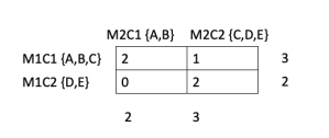
ARI is best understood using an example. So let's look at the example of two clustering results used earlier. Let's create a contingency table summarizing the results of two clustering methods. In this case, it is a 2x2 table wherein each cell of the table shows the number of times an example occurs in two clusters referenced by the corresponding row and column. M1C1 and M1C2 refer to two clusters formed by a hypothetical method-1. M2C1 and M2C2 similarly refer to two clusters formed by method-2. For clarity sake, I have included the examples forming the respective clusters next to M1C1, M1C2 etc. The top left cell has an entry of 2 because the clusters M1C1 and M2C1 share two examples, A and B. Entries in the other cells have similar meaning. The numbers to the right and below the contingency table show the sums along respective rows and columns.

To write the formula for ARI, lets generalize the entries of the contingency table using the following notation:

$n_{ij} = \text{Number of examples common to cluster i and cluster j}$

$a_i = \text{Sum of contingency cells in row i}$

$b_j = \text{Sum of contingency cells in column j}$

The ARI is then expressed as:

The first term in the numerator is known as index, and the second term as expected index. The first term in the denominator is called maximum index, and the second term of the denominator is same as the second term of the numerator. With these designations of the terms, the ARI is often expressed as

$\text{ARI} = \frac{\text{index - expected index}}{\text{maximum index - expected index}}$

Now lets go back to the contingency table for our example and calculate the different parts of the ARI formula first. We have:

$\sum_{ij}\binom{n_{ij}}{2} = \binom{2}{2} + \binom{1}{2} + \binom{0}{2} + \binom{2}{2} = (1 + 0 + 0 + 1)=2$

$\sum_i\binom{a_i}{2} = (\binom{3}{2}+\binom{2}{2}) = (3 + 1)=4$

$latex \sum_j\binom{b_j}{2} = (\binom{2}{2}+\binom{3}{2}) = (1 + 3) = 4$

Thus the index value for our example is 2; the expected index value is 1.6 (4*4/(5*4/2)). The maximum index value is 4. Therefore, the ARI for our example is (2 - 1.6)/(4 - 1.6), which equals 0.1666. We see that RI is much higher than ARI; this is typical of these indices. While RI always lies in 0-1; ARI can achieve a negative value also.

ARI is not the only measure to compare two sets of groupings. Mutual information based measure, adjusted mutual information (AMI), is also used for this purpose. May be in one of the future posts, I will describe this measure.

 

Linear Regression using ChatGPT

[Originally published on March 7, 2023]

The ChatGPT is a large language model (LLM) from OpenAI that was released a few months ago. Since then, it has created lots of excitement in terms of a whole range of possible uses for it, lots and lots of hype, and a lot of concern about harm that might result from its use. Within five days after its release, the ChatGPT had over one million users and that number has been growing since then. The hype arising from ChatGPT is not surprising; the field of AI from its inception has been hyped. One just need to be reminded of the Noble Prize winner Herbert Simon’s statement “Machines will be capable, within twenty years, of doing any work that a man can do” made in 1965. Several concerns about the potential harm due to ChatGPT’s use have been expressed. It has been found to generate inaccurate information as facts that is presented very convincingly. Its capabilities are so good that Elon Musk recently tweeted “ChatGPT is scary good. We are not far from dangerously strong AI.”

Since ChatGPT’s release, many companies and researchers have been playing with its capabilities and this has given rise to what is being characterized as Generative AI. It has been used to write essays, emails, and even scientific articles, prepare travel plans, solve math problems, write code and create websites among many other usages. Many companies have incorporated it into their Apps. And of course, Microsoft has integrated it into its Bing search engine.

Given all the excitement about it, I decided to use it to build a linear regression model. The result of my interaction with the ChatGPT are presented below. The complete interaction was over in a minute or so; primarily slowed by my one finger typing.

So, all it took to build the regression model was to feed the data and let the ChatGPT know the predictor variables. Looks like a great tool. But like any other tool, it needs to be used in a constructive manner. I hope you like this simple demo of ChatGPT’s capabilities. I encourage you to try on your own. OpenAI is free but you will need to register.

Words as Vectors

[This post was originally published on April 13, 2015.]

Vector space model is well known in information retrieval where each document is represented as a vector. The vector components represent weights or importance of each word in the document. The similarity between two documents is computed using the cosine similarity measure.

Although the idea of using vector representation for words also has been around for some time, the interest in word embedding, techniques that map words to vectors, has been soaring recently. One driver for this has been Tomáš Mikolov's Word2vec algorithm which uses a large amount of text to create high-dimensional (50 to 300 dimensional) representations of words capturing relationships between words unaided by external annotations. Such representation seems to capture many linguistic regularities. For example, it yields a vector approximating the representation for vec('Rome') as a result of the vector operation vec('Paris') - vec('France') + vec('Italy').

Word2vec uses a single hidden layer, fully connected neural network as shown below. The neurons in the hidden layer are all linear neurons. The input layer is set to have as many neurons as there are words in the vocabulary for training. The hidden layer size is set to the dimensionality of the resulting word vectors. The size of the output layer is same as the input layer. Thus, assuming that the vocabulary for learning word vectors consists of V words and N to be the dimension of word vectors, the input to hidden layer connections can be represented by matrix WI of size VxN with each row representing a vocabulary word. In same way, the connections from hidden layer to output layer can be described by matrix WO of size NxV. In this case, each column of WO matrix represents a word from the given vocabulary. The input to the network is encoded using "1-out of -V" representation meaning that only one input line is set to one and rest of the input lines are set to zero.

To get a better handle on how Word2vec works, consider the training corpus having the following sentences:

"the dog saw a cat", "the dog chased the cat", "the cat climbed a tree"

The corpus vocabulary has eight words. Once ordered alphabetically, each word can be referenced by its index. For this example, our neural network will have eight input neurons and eight output neurons. Let us assume that we decide to use three neurons in the hidden layer. This means that WI and WO will be 8x3 and 3x8 matrices, respectively. Before training begins, these matrices are initialized to small random values as is usual in neural network training. Just for the illustration sake, let us assume WI and WO to be initialized to the following values:

WI =

W0 =

Suppose we want the network to learn relationship between the words "cat" and "climbed". That is, the network should show a high probability for "climbed" when "cat" is inputted to the network. In word embedding terminology, the word "cat" is referred as the context word and the word "climbed" is referred as the target word. In this case, the input vector X will be [0 1 0 0 0 0 0 0]t. Notice that only the second component of the vector is 1. This is because the input word is "cat" which is holding number two position in sorted list of corpus words. Given that the target word is "climbed", the target vector will look like [0 0 0 1 0 0 0 0 ]t.

With the input vector representing "cat", the output at the hidden layer neurons can be computed as

Ht = XtWI = [-0.490796 -0.229903 0.065460]

It should not surprise us that the vector H of hidden neuron outputs mimics the weights of the second row of WI matrix because of 1-out-of-V representation. So the function of the input to hidden layer connections is basically to copy the input word vector to hidden layer. Carrying out similar manipulations for hidden to output layer, the activation vector for output layer neurons can be written as

HtWO = [0.100934 -0.309331 -0.122361 -0.151399 0.143463 -0.051262 -0.079686 0.112928]

Since the goal is produce probabilities for words in the output layer, Pr(wordk|wordcontext) for k = 1, V, to reflect their next word relationship with the context word at input, we need the sum of neuron outputs in the output layer to add to one. Word2vec achieves this by converting activation values of output layer neurons to probabilities using the softmax function. Thus, the output of the k-th neuron is computed by the following expression where activation(n) represents the activation value of the n-th output layer neuron:

Thus, the probabilities for eight words in the corpus are:

0.143073 0.094925 0.114441 0.111166 0.149289 0.122874 0.119431 0.144800

The probability in bold is for the chosen target word "climbed". Given the target vector [0 0 0 1 0 0 0 0 ]t, the error vector for the output layer is easily computed by subtracting the probability vector from the target vector. Once the error is known, the weights in the matrices WO and WI

The probability in bold is for the chosen target word "climbed". Given the target vector [0 0 0 1 0 0 0 0 ]t, the error vector for the output layer is easily computed by subtracting the probability vector from the target vector. Once the error is known, the weights in the matrices WO and WI

can be updated using backpropagation. Thus, the training can proceed by presenting different context-target words pair from the corpus. In essence, this is how Word2vec learns relationships between words and in the process develops vector representations for words in the corpus.

Continuous Bag of Words (CBOW) Learning

The above description and architecture is meant for learning relationships between pair of words. In the continuous bag of words model, context is represented by multiple words for a given target words. For example, we could use "cat" and "tree" as context words for "climbed" as the target word. This calls for a modification to the neural network architecture. The modification, shown below, consists of replicating the input to hidden layer connections C times, the number of context words, and adding a divide by C operation in the hidden layer neurons. [An alert reader pointed that the figure below might lead some readers to think that CBOW learning uses several input matrices. It is not so. It is the same matrix, WI, that is receiving multiple input vectors representing different context words]

With the above configuration to specify C context words, each word being coded using 1-out-of-V representation means that the hidden layer output is the average of word vectors corresponding to context words at input. The output layer remains the same and the training is done in the manner discussed above.

Skip-Gram Model

Skip-gram model reverses the use of target and context words. In this case, the target word is fed at the input, the hidden layer remains the same, and the output layer of the neural network is replicated multiple times to accommodate the chosen number of context words. Taking the example of "cat" and "tree" as context words and "climbed" as the target word, the input vector in the skim-gram model would be [0 0 0 1 0 0 0 0 ]t, while the two output layers would have [0 1 0 0 0 0 0 0] t and [0 0 0 0 0 0 0 1 ]t as target vectors respectively. In place of producing one vector of probabilities, two such vectors would be produced for the current example. The error vector for each output layer is produced in the manner as discussed above. However, the error vectors from all output layers are summed up to adjust the weights via backpropagation. This ensures that weight matrix WO for each output layer remains identical all through training.

In above, I have tried to present a simplistic view of Word2vec. In practice, there are many other details that are important to achieve training in a reasonable amount of time. At this point, one may ask the following questions:

1. Are there other methods for generating vector representations of words? The answer is yes and I will be describing another method in my next post.

2. What are some of the uses/advantages of words as vectors. Again, I plan to answer it soon in my coming posts.