What is Neuro-Symbolic AI and Why do we Need it?

Neuro-symbolic AI, also known as symbolic neural integration or hybrid AI, has been in news lately. It is an approach that combines symbolic reasoning and neural networks to create more robust and flexible artificial intelligence systems. This integration aims to leverage the strengths of both symbolic and neural approaches, addressing some of the limitations each paradigm faces independently.

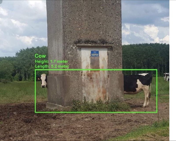
Let's look at the following image to understand the need for the neuro-symbolic approach. The deep learning model looking at the input image comes to a conclusion that the image depicts a cow that is 5.2 meter long. Obviously, the system has been trained to recognize cows and other objects but is unable to reason that cows are not that long. This is not surprising as deep learning models are excellent at recognizing features but have no capability to understand or draw conclusions based on the spatial relationships between the detected features. One way to provide such capabilities is to integrate symbolic reasoning along with the feature detection and pattern recognition capabilities of deep neural networks, and thus the interest in the neuro-symbolic approach. 

#object detection #neuro-symbolic

The ways Neuro-Symbolic AI can help

  1. Improved Reasoning: Integrating symbolic reasoning with neural networks can enhance AI's ability to understand and apply common sense knowledge, making it more adept in real-world scenarios.
  2. Medical Diagnosis: Neuro-symbolic approaches can be applied to medical diagnosis, where symbolic rules can be used to represent expert knowledge, and neural networks can learn from diverse patient data to improve diagnostic accuracy.
  3. Robotics and Autonomous Systems: Combining symbolic reasoning with neural networks can enhance the decision-making capabilities of robots, allowing them to navigate complex environments and handle uncertainty.
  4. Natural Language Understanding: Neuro-symbolic AI can be used to improve natural language understanding systems by combining semantic representation with the ability to learn from diverse textual data.
  5. Financial Fraud Detection: Integrating symbolic rules for detecting fraud patterns with neural networks that can adapt to new, emerging fraud trends can enhance the accuracy and robustness of fraud detection systems

Challenges and Approaches

Integrating the neural and symbolic components in a principled and effective way remains a key challenge in neuro-symbolic AI. Several promising approaches are being explored:
  1. Neural Networks with Symbolic Inductive Biases: This approach aims to build neural architectures with inductive biases derived from symbolic AI, such as logical operations, algebraic reasoning, or compositional structure. For example, graph neural networks can inject relational inductive biases, while neural programmer-interpreters combine neural modules with program-like operations.
  2. Augmenting Neural Models with External Memory/Reasoning: Rather than directly encoding symbolic knowledge in the neural architecture, another approach uses external memory or reasoning components that interact with a neural network. Examples include memory augmented neural networks, neural semantic encoders, and neural-symbolic concept learners.
  3. Differentiable Inductive Logic Programming: Inspired by inductive logic programming (ILP) in symbolic AI, this approach uses neural networks to learn first-order logic rules or program-like primitives in a differentiable way that integrates symbolic reasoning into end-to-end training.
  4. Learning Symbolic Representations from Data: Techniques in this area aim to have neural networks automatically learn disentangled, symbolic-like representations from raw data in an unsupervised or self-supervised manner. Examples include sparse factor graphs, conceptor-based models, and neuro-symbolic concept invention.

For Further Exploration

You can check the following links for further exploration of this topic:
Despite progress, several key challenges remain, including scaling symbolic reasoning, imposing harder constraints in neural architectures, achieving systematic compositionality, and maintaining interpretability as models get larger. Hybrid neuro-symbolic approaches hold promise but will require significant research efforts across multiple fields.

More on Distances between Graphs

In an earlier post, I had mentioned the need for comparing graphs for different applications and described the spectral graph distance for the said purpose. In this post, we are going to consider two other graph distance measures. The first measure is called DeltaCon measure. This measure works under the assumption that the node correspondence between the two graphs is known. The second measure is known as the Portrait Divergence and can be used for any graph pair. In addition to these two measures, there are a few other measures that are available. It turns out that most measures yield highly correlated results; thus knowing 2-3 different measures is a good starting point to explore other measures as well as the applications where such measures are used.

DeltaCon Measure of Graph Similarity

The basic idea behind this method is to calculate an affinity measure between a pair of nodes in the first graph, repeat the similar affinity calculations for the corresponding node pair in the second graph, and then compare the two measures to get an idea about the difference in the node pairs over two graphs. By repeating the node affinity calculations over all node pairs for the respective graphs, one can get an aggregate measure for similarity between the two graphs. The pairwise node affinity s_{ij} between node I and node j is measured by looking at all possible paths between the two nodes. The DeltaCon paper shows that the similarity matrix S of a graph G measuring the similarity between different node pairs can be obtained by the following expression:

S = [s_{ij}] = [I + \epsilon^2 D - \epsilon A]^{-1},

where I is an identity matrix, D is the degree matrix, and A is the adjacent matrix of the graph G. The quantity \epsilon is a small positive constant.Given two graphs G^1 and G^2, the DeltaCon distance measure is computed using the following relationship:
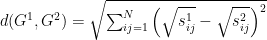
d(G^1,G^2) = \sqrt{\sum_{ij=1}^N\Big(\sqrt{s_{ij}^1}- \sqrt{s_{ij}^2}\Big)^2}

While the two similarity matrices can be compared using some other difference measure, the above DeltaCon measure is a true metric satisfying the triangular inequality of a true distance.

Illustration of DeltaCon Measure

Let’s use DeltaCon measure to compute distances between a set of graphs. We will do this using the netrd library which provides a NetworkX-based interface to compute various graph distances along with many other graph utilities. We will use the Air Transportation Multiplex Dataset for experimentation. The dataset is composed of a multiplex network composed of the airlines operating in Europe. It contains thirty-seven different layers of networks each one corresponding to a different airline. We will use only two subsets of the dataset consisting of the three biggest major airlines (Air France, British Airways, and Lufthansa),  and the three low-cost airlines (Air Berlin, Easy Jet, and Ryanair). A graph of the Ryanair is shown below; it consists of 149 nodes with 729 edges.

Ryanair Network
All the nodes in the dataset have an associated airport code and node indices are consistent over the entire multiplex. Thus, the node correspondence exists in the dataset. However, each airline flies to only a subset of the total nodes in the multiplex. Since DeltaCon requires node correspondence as well the same number of nodes in the two graphs to compare, we need to add nodes to the graphs under comparison to bring them to same size. The following code snippet shows how the DeltaCon distance is being computed for a pair of airlines; similar computation applies to other airline pairs.

import numpy as np
import networkx as nx
import netrd 

f = nx.read_adjlist(France.txt)
Fr = nx.Graph(f)
b = nx.read_adjlist(Brit.txt)
Br = nx.Graph(b)
list1 = list(Fr.nodes)
list2 = list(Br.nodes)
new_list1=set(list1)-set(list2)#Elements of list 1 that are not present in list 2
new_list2=set(list2)-set(list1)#Elements of list 2 that are not present in list 1 
Fr.add_nodes_from(new_list2)
Br.add_nodes_from(new_list1)
# Now both graphs have identical size and nodes are in correspondence
dist = netrd.distance.DeltaCon()
print(dist(Fr,Br))
1.5233983011182537

The figure below shows the distances between the networks of different airlines calculated using the DeltaCon measure. I applied the single linkage clustering to the resulting distance. The result shown below in the form a dendrogram puts the three major airlines in one cluster and the three low-cost airlines in another cluster. This suggests that the DeltaCon distance is able to capture the underlying properties of a graph and can be used for graph discrimination.

Distance matrix and Dendrogram by using DeltaCon

Portrait Divergence

This measure is based upon a matrix, called network portrait, which captures the distribution of shortest path lengths in a graph. The elements of the network portrait matrix $B$ for a graph with N nodes are defined as

$b_{j,k} \equiv \text{the number of nodes who have k nodes at distance j}$,

$ \text{ for } 0 ≤ j  ≤ D \text{ and } 0 ≤ k ≤ N − 1$. The distance is taken as the shortest path length and D refers to the graph diameter(length of the longest shortest path). The network portrait provides a concise topological summary of a graph and has the graph invariant property, and thus can be used for comparing two networks or graphs.

The portrait divergence measure is computed by treating the rows of the network portrait matrix B as probability distributions. These probability distributions are combined to create a single joint distribution for all rows. Given two graphs, the corresponding distributions are then compared using the Jensen-Shanon divergence measure to produce a similarity value in the range of 0-1. Please see for details.

Let’s see if the results given by this method are different from above or not by applying the portrait divergence measure to the airlines data. The results are shown below; these are similar and yield two similar clusters.

Distance matrix and Dendrogram by using Portrait Divergence

Takeaway

I have discussed only three methods for graph comparison, spectral graph distance (in an earlier blog post) and the two discussed in this post. The DeltaCon method requires prior knowledge about the graphs in terms of node to node mappings over the graph pair being compared. The spectral graph distance and the portrait divergence methods do not have any such requirement. As I indicated earlier, there are a few other distance measures for graph comparison; however all these measures yield correlated results. I suggest looking at this paper if you get interested in this topic as a result of this post.


Measuring Distance between Two Graphs

Graph-based representation is a natural choice in many areas such as biology, computer science, communication, social sciences, and telecommunication. Such representations are also known as network models. Often, we are interested in finding out how much different the two graphs are and want to specify that difference in the form of a numerical measure such as the distance or similarity between a pair of graphs. Measuring the distance between two graphs is different from the graph isomorphism problem where we look for a mapping based on one-to-one correspondence between the nodes of the two graphs. In this blog post, I am going to describe the graph distance measure, spectral graph distance, which has been suggested and used to measure the difference between a pair of graphs. In the subsequent blog posts, I intend to describe some other graph distance/similarity measures. 

Graph Basics

Before describing the spectral graph distance, let’s take a look at some basic definitions related to graphs. A graph is represented as G(V, E) where V represents a list of vertices/nodes and E represents a list of edges between those nodes. The adjacency matrix A of a graph is matrix of size |V|x|V| where |V| is the number of vertices or nodes in the graph. The element $a_{ij}$ of the adjacency matrix is 1 if there is an edge between the vertex-i and vertex-j; otherwise it is 0. This is true for undirected graphs without weights assigned to edges. An example of a graph G and its adjacency matrix are shown below.

An example graph with its adjacency matrix

The degree of a node is the number of edges with the node. The degree matrix, D, is used to convey the degree information for all the nodes in a graph. The degree matrix is a diagonal matrix where $d_{ii}$ equals the degree of the i-th node. For the graph shown above, the degree matrix is as shown below:


Another matrix of interest is the Laplacian matrix of a graph. It is defined as L = D – A. The Laplacian matrix is known to capture many useful properties of a graph. The Laplacian matrix of an undirected graph is a symmetric matrix and so is the adjacency matrix. The Laplacian matrix for the above example graph is given as

Spectral Graph Distance

The eigenvalues of the graph matrices, adjacency or Laplacian, provide information about the graph’s structural properties, such as the number of connected components, the density of the graph, and the distribution of degrees. Thus, comparing two sets of eigenvalues coming from two different graphs, we can compute the distance between them. Such a distance measure then can be used for various graphs related tasks, for example for clustering graphs or monitoring changes in a graph over time. The comparison between the two sets of eigenvalues is done by sorting the respective eigenvalues in descending (for adjacency matrices) or ascending (for Laplacian matrices) order. The sorted eigenvalues of a matrix define its spectrum. For example, the spectrum of the above adjacency matrix is 3.323 ≥ 0.357 ≥ -1 ≥ -1 ≥ -1.681, while the Laplacian matrix spectrum is 0 ≤ 2 ≤ 4 ≤ 5 ≤ 5.

The Laplacian matrix is preferred for calculating the spectral graph distance because of its properties. The Laplacian matrix of an undirected graph is a positive-semidefinite matrix and thus its eigenvalues are all positive. Further, the sum of every row or column is 0 and thus the smallest eigenvalue is always 0. The number of eigenvalues equal to 0 indicates the number of connected components in the graph. It turns out that the presence of a vertex with a high degree of connectivity tends to dominate the Laplacian matrix. To avoid this, it is common to normalize the Laplacian matrix. The normalized Laplacian matrix is defined as

\bf{\mathcal{ L} }= {D^{-1/2}LD^{-1/2}},

where the diagonal components of the matrix D^{-1/2} are given as 1/\sqrt{d_{ii}}
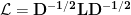
and non-diagonal components being zero. The following is the normalized Laplacian of the matrix L shown earlier.


Generally, we use only k eigenvalues to compute the graph distance. Thus, given two graphs G_1 and G_2, the spectral graph distance will be computed as

D(G_{1}, G_{2}) = \sqrt{\sum_{i=1}^{k} (\lambda_i^{g_1} - \lambda_i^{g_2})^2}

The spectral distance using adjacency matrix or any other matrix is computed similarly. 

Illustration of Spectral Graph Distance

Let’s now use the spectral graph distance on a small set of well-known graphs. We will compute the distance between different graph pairs to generate an inter-graph distance matrix. The following graphs are used.

  • American College Football
  • Les Miserables
  • Protein Network
  • Dolphins
  • Yeast
  • Celegans

These datasets were downloaded from network repository.com and the network data site. Three of these graphs, Football, Les Miserables, and Dolphins, are the social network graphs. The Protein Network and Yeast are biological graphs, and Celegans is a metabolic network.

I used the Netcomp package to do the distance computations. For no particular reason, I used the truncated spectra of 16 components. The inter-graph distance matrix and the resulting dendrogram using single link analysis are shown below. we can see that the spectral graph distance is able to cluster the social network graphs separately from the biological networks while the metabolic network, Celegans, is a cluster by itself.

The spectral graph distance is not the only method for computing distances between graphs; there are a few other methods as well. I hope to describe them in future posts.

Before you leave, please note that the spectral graph distance is not a metric. It doesn’t satisfy triangular inequality.